
Abstract
In this paper, a representational framework is presented featuring a qualitative notion of similarity. It is aimed at issues of natural language semantics, in particular the semantics of expressions of similarity and sameness and their role in comparison and ad-hoc kind formation. The framework makes use of attribute spaces, which are well-established in AI and also in some branches of natural language semantics, e.g., frame-based approaches (Barsalou 1992). What distinguishes attribute spaces and representations as proposed in this paper is the idea of systems of predicates on attribute spaces corresponding to predicates on the domain. On the worldy side, a domain includes a set of relevant predicates talking about individuals. These predicates have counterparts on the representational side talking about points of an attribute space. Counterpart predicates are required to be consistent with their originals; more precisely, they have to agree in truth-value on the set of positive and negative exemplars thereby approximating the original predicates. Moreover, counterpart predicates will be assumed to have convex and open extensions. This system facilitates a qualitative notion of similarity which is suited to account for the meaning of natural language similarity expressions and, furthermore, their role in comparison and ad-hoc kind formation.
You have full access to this open access chapter, Download chapter PDF
1 Introduction
In this paper, a representational framework is presented featuring a qualitative notion of similarity. It is aimed at issues of natural language semantics, in particular the semantics of expressions of similarity and sameness and their role in comparison and ad-hoc kind formation.Footnote 1 Starting point was the interpretation of such expressions in German and English, for example so/such, ähnlich/similar, and gleich/same, which all denote similarity in some sense. It would be unsatisfactory, however, to treat similarity as a primitive predicate because semantic differences between individual similarity expressions would be obscured, for example, the fact that ähnlich/similar are gradable while so/such and gleich/same are not (see Umbach and Gust in print). Furthermore it would be difficult to establish the connection between similarity expressed by scalar and non-scalar equative comparison constructions, as shown in (1).
(1) | a. | Anna is as tall as Berta. | scalar/adjectival |
b. | Anna has a car like Berta’s. | non-scalar/nominal | |
c. | Anna is dancing just like Berta. | non-scalar/verbal |
Finally, a primitive similarity predicate would leave no room to account for the observation that certain similarity expressions, in certain contexts, can be used to form ad-hoc kinds. German so as well as English such combined with nominal expressions may refer to kinds (or concepts) instead of individuals. In (2a, b), for example, so ein Fahrzeug/such a vehicle does not refer to a particular vehicle but instead to an ad-hoc created kind of vehicles including the set of vehicles similar to the one the speaker points to. Umbach and Stolterfoht present experimental exidence that features licensing ad-hoc kinds must be principally connected to concepts, excluding factual and statistical properties (König and Umbach 2018; Umbach and Gust 2014; Umbach and Stolterfoht in prep.). Thus, a complex notion of similarity not only provides a detailed semantic interpretation of natural language similarity expressions—it opens a window into mechanisms of concept formation.
(2) | (Speaker points to an oversized car that makes enormous noise:) | |
a. | So ein Fahrzeug wird in den Innenstädten bald verboten sein. | |
b. | Such a vehicle will soon be banned in the inner cities. | |
The framework in this paper offers a way to spell out the notion of similarity in some detail without being forced to leave the well-established ground of referential semantics. The core idea is to make use of attribute spaces representing complex features of individuals, and to make use of predicates defined on such features determining the granularity of representation. In accordance with referential semantics we assume that natural language expressions refer to entities, or categories of entities, in the real world. However, access is only indirect, mediated by generalized measure functions mapping real world entities to points in attribute spaces (this is called a mediated reference theory in Färber, Svetashova and Harth, this volume). Similarity is a key concept in our framework because it provides a variable notion of identity/indistinguishability with respect to a representation: Individuals count as similar if their features in a particular attribute space, given a particular granularity, cannot be distinguished.
This system provides a powerful and flexible tool in the analysis of natural language semantics facilitating detailed interpretations of similarity expressions (so, such, similar etc.). Beyond, and maybe even more relevant, this system offers the possibility to analyze linguistic ad-hoc kind formation constructions, for example, by so/such demonstratives and equative comparison as in (1) and (2). It is important to realize, however, that this system is basically a multidimensional generalization of degree semantics (e.g., Kennedy 1999) complemented by a method for varying granularity. From this point of view, our framework is anchored in referential semantics just as much as degree semantics is.
Attribute spaces are well-established methods of representation in AIFootnote 2 and also in some branches of natural language semantics, e.g., in frame-based approaches (Barsalou 1992; Minsky 1975). What distinguishes attribute spaces and representations as proposed in this paper from classical frame-based approaches is that we focus on systems of predicates on points in attribute spaces in contrast to the points in these spaces themselves, thereby introducing a qualitative aspect, for instance in modelling comparison. This idea is connected to the idea of micro-theories (see, e.g., in CycFootnote 3 or other ontology languages) which talk about small parts of the world covered, e.g., by a single concept like chair, vehicle, elephant, human, etc., but also about actions and events. We expect that such micro-theories provide some kind of prototypes or exemplars, positive and also negative ones. Maybe we just imaginate such exemplars. Here is a typical way how to introduce the concept of a physical object in a beginners lecture in experimental physics by imagination of a positive exampleFootnote 4: “Think of a red steel ball of ten centimeters diameter in front of you. It need not to be red, it need not to be made from steel, it need not have a diameter of ten centimeters and it need not be a ball.” This shows that even abstract concepts can be characterized by exemplars (real or imaginated) together with the specification of relevant dimensions in an attribute space.
This paper is structured in the following way: In Sect. 2 we develop a formal theory of representation making use of predicate systems over attribute spaces. Section 3 gives a brief overview over the interpretation of natural language similarity expressions and the role of similarity in ad-hoc kind formation and equative comparison. Since the focus of this paper is on formal characteristics of the representational framework, we will not go into linguistic details.Footnote 5 In Sect. 4 we develop a formal similarity concept based on methods provided in Sect. 2. Section 5 shows how to use granularity and hierarchies of representations in order to model gradabilty along non-scalar dimensions.
2 Representations in Multi-dimensional Attribute Spaces
We start from the idea that natural language expressions refer to entities or categories (or even higher order structures, e.g., relations) of entities in the real world, but in an indirect way. Access to these entities or categories is mediated by a function we call generalized measure function, e.g., car1 ⇒ {horse_power: 100 ps, weight: 1680 kg, color: green …}. This is related to what is called observables in physicsFootnote 6: Such a function assigns observable attributes (elements of an attribute space) to entities or classes of entities in the world.Footnote 7 The referential power of language predicates like car (their meaning in the world) can thus be approximated by classifiers. Such classifiers should be effectively computable characteristic functions of predicates.Footnote 8 They operate on attribute spaces (or higher order structures based on attribute spaces).Footnote 9 Still, we can go back from predicates on points in attribute spaces to predicates on the entities in the world via the inverse image of the generalized measure functions.
On the worldy side, a domain includes a set of relevant predicates P talking about entities in the world. According to the notion of a representation in this paper, these predicates have counterparts on the representational side marked by a star (*) in Fig. 1. Counterpart predicates are required to be consistent with their originals; more precisely, they have to agree in truth value on the set of positive and negative exemplars of the original predicate. Moreover, counterpart predicates will be assumed to have convex extensions. As a consequence, they must be true on all points in the convex closure of the images of the positive exemplars (see Fig. 1 below). In addition, we stipulate that the extensions of counterpart predicates must be openFootnote 10 in some given topology on attribute spaces. This ensures that small changes in the representation (in the sense of the given topology) do not change the truth-values of these predicates.

A domain of vehicles and a representation featuring positive and negative exemplars of small cars
2.1 Domains and Representations
We start the formalization of our approach by introducing domains and representations. For classifiers, given the truth-value true, we get the extension in the attribute space by its inverse image of {true}, and we get its extension in the real world by applying the inverse image of the measure function. However, given a language predicate like small in the context of cars, its reference will in general not be completely determined by a classifier small*car and by subsequently applying the inverse image of the measure function. An entity which has all the attributes of a small car may not be a small car, and an entity which is a small car may not have all the attributes we in general assign to cars. In this sense, classifiers approximate the denotation of language predicates. This approximation relation is subject to consistency constraints: If we know that x is a small car and y is similar enough to x, we expect that y is a small car, too. What should ‘similar enough’ mean? In our approach, we can express this in terms of the attribute space: The attribute values must be similar enough.
If the classifiers cannot discriminate between the representations (points in the attribute space) of two entities x and y, they must belong to the same concepts: If one is a small car, then the other must be a small car, too. In particular, this is the case if the representations in the attribute space are equal. Think of a situation where we measure size only with very low precision or specify color only by a few color values. If the above constraint is violated we should probably change our attribute space and/or our measure function, e.g., increase precision of measuring size and/or introduce a more fine-grained color specification.
Often we have additional structure on our attribute space, e.g., a (pre)order relation. Assume that x and y are small cars, and z is in the car domain. The number of wheels are wx, wy, wz respectively; x, y, and z differ only in the number of wheels. Then, if wx ≤ wz ≤ wy we expect z to be a small car, too. If not, we again have an inconsistency in our representation. And again, we probably should change it. The mathematical foundation of this type of inconsistency is the theory of convex closures. The formal definition of a convex closure operator cl on a set X is the following (see Korte et al. 1991):
A function cl: ℘(X) → ℘(X) is a convex closure operator iff
• it preserves the empty set | cl({}) = {} |
• it is extensive | A ⊆ cl(A) for all A ⊆ X |
• it is monotone | A ⊆ B → cl(A) ⊆ cl(B) |
• it is idempotent | cl(cl(A)) = cl(A) |
• the anti-exchange property holds | x, y ∉ X, x ≠ y, x ∈ cl(X ∪ {y}) → y ∉ cl(X ∪ {x}) |
In the two-dimensional Euclidean plane, we can visualize the effect of a convex closure operator. Suppose X is cl({a, b, c}). If x is in cl(X ∪ {y}), then y cannot be in cl(X ∪ {x}). The anti-exchange property ensures convexity. In a two-dimensional Euclidean plane, this means that for any two points in X the connecting line must also be in X (Fig. 2).

Convex closure and anti-exchange property in the Euclidean plane
On a (partially) ordered set (M, ≤) we can define convex closure operators in a natural way (see Fig. 3). For A ⊆ M we define:
left closure: | cl←(A) = {x ∈ M | ∃ y ∈ A: x ≤ y} |
right closure: | cl→(A) = {x ∈ M | ∃ y ∈ A: y ≤ x} |
convex closure: | cl(A) = {x ∈ M | ∃ y, z ∈ A: y ≤ x ≤ z} |
To sum up: We approximate the meaning of natural language predicates by classifiers and their inverse images by means of a generalized measure function. Additionally, we request that classifiers respect some consistency constraints: (i) they should classify known examples correctly, (ii) their extension (as a subset of the attribute space) should be convex according to a suitable convex closure operator and (iii) their extensions should be open in a suitable topology. The topology and the closure operator must be compatible: Closures of open sets must be open.
First, we need a notation to refer to the entities we are talking about by a natural language predicate like small car: the set of entities (in the world) for which it makes sense to ask if they have car properties, that is, entities for which the attribute dimensions for cars make sense, e.g., number of wheels, horsepower, size, weight, color etc. We exclude entities for which it does not make sense to ask if they have car properties, e.g., single atoms, trees, hens etc.
Next, we assume that we have clear cases: positive examples such as entities which are definitely cars, and negative examples such as entities for which the attribute dimensions of cars make sense but which are definitely not cars, e.g., motorbikes. Concepts which are related and belong to the same micro-theory are collected as predicates over the same domain. Think of different types of cars, bikes, trikes etc.
We assume that there is a universe U which includes all the entities in the world. We can start now formalizing our approach by defining a domain as a subset of the universe U together with a set of predicates and non-overlapping sets of positive and negative examples for each predicate.

A non-convex set in the two-dimensional plane and its convex closure
Definition 1
Domain
A domain \(\mathcal{D}\) is a quadruple 〈\(D,\) _\(^{+},\) _−, P〉 with:
• D ⊆ U | a set of individuals/entities (called the carrier of the domain), |
• P = {p1, … pn} | a set of identifiers of predicates over D, |
• _D: P ⟶ ℘(D) | the extension in D of a predicateFootnote 11 denoted by index DFootnote 12 |
• _+: P ⟶ ℘(D) | a function which assigns a set of positive examples to each predicate (\(\text{for}\) _+ (p) we write p+), |
• _−: P ⟶ ℘(U) | a function which assigns a set of negative examples to each predicateFootnote 13 ( $$\text{for}$$ for _− (p) we write p−), |
• ∀p ∈ P: pD+ ∩ pD− = ∅ (consistency), | |
• ∃q ∈ P ∀p ∈ P: pD+ ⊆ qD+ ∧ pD− ⊆ qD+ ∧ qD− ∩ D = ∅ (universal predicate). | |
2.2 Representations and Classifier Systems
We view the elements of D as entities to which we have only indirect access via a (generalized) measure function μ. The measure function μ constructs representations of the entities in D as points in an attribute space F, much like observables in physics. Attribute spaces are well-established representational structures.Footnote 14 They generalize vector space approaches in allowing heterogeneous dimensions equipped with value sets of different scales (nominal, ordinal, interval, proportional, partially ordered etc.), where value sets may themselves be attribute spaces with multiple dimensions.
An attribute space F is given by a set of attributes A = {a1, …, an}, such that for each ai in A there is a set of possible values Vai of ai. Elements of D are mapped to points in \(V_{a1}\times\cdots\times V_{an}\), the carrier of the attribute space F. Think, for example, of number of wheels as an attribute with {1, 2, 3, 4, 5, 6, …} as its value set, or horsepower as an attribute with the positive real numbers as its value set.Footnote 15
A representation includes an attribute space F, a (generalized) measure function μ mapping elements of a domain into the attribute space, and a set of classification functions p* applying to points in the attribute space. In the case of the attribute number of wheels the measure function μ just has to count. In the case of the attribute horsepower a complex measurement procedure is required to determine the value of μ. The classification functions (short classifiers) serve as approximationsFootnote 16 of the predicates in P.Footnote 17 Moreover, the extensions of the classifiers will be assumed to be open and convex. This means that F comes with a convex closure operator cl and p* must be true on cl(μ(p+)).Footnote 18 Using the n-dimensional Euclidean space as an example, the extensions of the classifiers must not have holes, notches or coves in the representation space F.
Definition 2
Representation
A representation \(\mathcal{F}\) = \(\langle\langle\)F, cl\(\rangle, \mu,\) _*, \(\mathcal{D}\)〉 of a domain \(\mathcal{D}\) = \(\langle D,\) _+, _−, P\(\rangle\) is given by
-
an attribute space F together with a closure operator cl and a compatible topology (we write F for \(\langle\)F, cl\(\rangle\) if we are not interested in the closure operator cl),
-
a measure functionFootnote 19 μ: D → F,
-
a function _*: P → ΩF
(we write p* for _*(p) and call them classifiers).Footnote 20
Representations are subject to three consistency constraints:
-
∀p ∈ P the extension of p* must be open and convex in 〈F, cl〉
-
∀p ∈ P ∀x ∈ p+: p*(μ(x)) = true
-
∀p ∈ P ∀x ∈ p− ∩ D: p*(μ(x)) = false
From this we get μ(pi+) ∩ μ(pi− ∩ D) = ∅ (Fig. 4).

Domains and representations
As mentioned above, attribute spaces are familiar methods of representation. What distinguishes attribute spaces from the representations proposed in this paper is the idea of classifiers on attribute spaces. On the worldy side, a domain includes a set of relevant predicates p ∈ P. On the representational side, these predicates have counterparts, namely classifiers p* ∈ P*. By P* we denote the set of all basic classifiers: P* = {p* | p ∈ P}. These classification functions are required to be consistent with their corresponding predicates over D; more precisely, for the set of positive/negative exemplars the truth-values of the classification functions have to agree with the truth-values of the original predicates (see Definition 2).
Given a set of basic classifiers,Footnote 21 we assume the possibility to construct derived classifiers by logical operations: For the logical conjunction this is unproblematic (convex sets and open sets are closed under intersection). For the logical disjunction we have to apply the convex closure operator cl to the result. For negation this is not possible. Thus we do not allow to define complex classifiers by applying negation to elementary ones.Footnote 22 We name the set of derived classifiers \(\tilde{P}^*\).
Definition 3
Classifier systems
Given a set of basic classifiers B over an attribute space F, we define a set of classifiers \(\tilde{B}\) inductively (much like a topology):
• B ⊆ \(\tilde{B}\) | we expect that elements of B are convex and open, |
• X ∈ \(\tilde{B}\), Y ∈ \(\tilde{B}\) → X ∩ Y ∈ \(\tilde{B}\) | intersections, |
• X ∈ \(\tilde{B}\), Y ∈ \(\tilde{B}\) → cl ( X ∪ Y) ∈ \(\tilde{B}\) | closures of unions. |
If F is (partially) ordered:
• X ∈ \(\tilde{B}\) → cl→(X) ∈ \(\tilde{B}\quad{}{cl}\)→(X) = {x ∈ F | ∃ y ∈ X: y ≤ x} | right closures, |
• X ∈ \(\tilde{B}\) → cl←(X) ∈ \(\tilde{B}\quad{}{cl}\)←(X) = {x ∈ F | ∃ y ∈ X: x ≤ y} | left closures. |
It is important to mention that in general \(\tilde{B}\) is not closed under complement. This means that we do not have negation: Complements of convex sets need not be convex and complements of open sets need not be open. We start with basic classifiers B = p* = {p1*, …, pn*} and get \(\tilde{P}^*\) as the corresponding system of classifiers.
3 Similarity Expressions in Natural Language
In this section, a brief overview will be given of the challenges involved in the interpretation of similarity expressions. This section will not give a full description of the semantic phenomena—references will be given for details—but instead serve as a motivation for the specifics of the similarity framework presented in this paper.
3.1 Similarity Demonstratives
The need for a framework that models similarity originated from the problem of how to interpret the German demonstrative so (‘so’/‘such’). It is a genuine demonstrative expression, so we expect direct reference in the sense of Kaplan (1989). It does not, however, express identity as does, e.g., dies/this, and instead it refers to a set of entities which are in some sense similar to the target of the demonstration gesture (the entity the speaker points to). If the speaker points to a car while uttering “So ein Auto hat Anna” (‘Anna has a car like this’), Anna’s car is said to be, with respect to a particular set of features, indistinguishable from the car the speaker points to. This kind of demonstrative expressions is called similarity demonstratives in Umbach and Gust (2014), Gust and Umbach (2015), and demonstratives of manner, quality and degree in König and Umbach (2018).
We follow Nunberg’s (1993, 2004) adaptation of the Kaplanian analysis, interpreting demonstratives as directly referential expressions, but at the same time dismissing the idea that the target of the demonstration is necessarily identical to the referent of the demonstrative. This allows for a straightforward interpretation of similarity demonstratives such that the target of the demonstration is the individual or event the speaker points to, and the referent of the demonstrative phrase is related to the target by similarity instead of identity. Similarity is then implemented by indistinguishability of points in attribute spaces (see Sect. 4). This implementation of similarity is in fact close to the idea of contextual granularization suggested in Nunberg (2004): When restricting attention to a particular set of features, it may be the case that two entities can no longer be distinguished. It is important to note, however, that this idea requires a framework that distinguishes between a referential and a representational level—you cannot speak about indistinguishability without access to what could have been distinguished.
3.2 Ad-Hoc Kinds
According to the similarity analysis, demonstratives like German so and English such create classes of similar items, e.g. similar cars. There is some evidence that in the nominal and verbal case (though not in the adjectival case) these similarity classes constitute ad-hoc kinds. In a nut-shell, so/such phrases can be shown to be restricted to particular features of comparison. For example, the feature number of doors would be perfect when comparing cars but not when comparing mugs—mugs do not have doors, so the number of doors does not qualify as a feature of comparison for mugs. But mugs as well as cars can be recently purchased and nevertheless being recently purchased does not qualify as a feature of comparison for neither cars nor mugs. This suggests that properties qualifying as features of comparison must not be accidental.
There is experimental evidence that features of comparison are restricted to properties which are neither accidental nor evaluative (see König and Umbach 2018; Umbach and Stolterfoht in prep.). This raises the question of how to characterize these properties, which is a prominent issue in the debate about concept formation in cognitive psychology. Only recently has this debate been connected to the topic of genericity in linguistics by Greenberg (2003) and Carlson (2010), and by the experimental studies in Prasada and Dillingham (2006) and Prasada et al. (2013), providing evidence that there are so-called principled connections between kinds and properties that an entity has, because it is the kind of thing it is.
There is an alternative analysis claiming that demonstratives like German so and English such are pro-kind expressions (see Anderson and Morzycki 2015, adapting Carlson’s 1980 kind-referring analysis of such). The final results of the two accounts are fairly close. However, unlike the pro-kind account, the similarity account not just postulates that so/such phrases denote kinds, but in addition shows how these kinds emerge, namely by similarity.
3.3 Equative Comparison
Another phenomenon where similarity plays a significant role is equative comparison, including non-scalar as well as scalar cases, see (3a–c).Footnote 23 In German, scalar as well as non-scalar equatives are uniformly constructed by so … wie where so is a correlative pronoun relating to the standard of comparison given in the wie clause:
(3) | a. | Anna ist so groß wie Berta Anna is as tall as Berta | scalar/adjectival |
b. | Anna hat so ein Auto wie Berta Anna has a car like Berta’s | non-scalar/nominal | |
c. | Anna tanzt so wie Berta Anna is dancing just like Berta | non-scalar/verbal |
Given that the demonstrative so can in general be substituted by wie dies (‘like this’), it suggests itself to analyze wie as expressing similarity as does so, though without a deictic component. This allows for a generalized account of equative comparison: The nominal equative in (3b) is interpreted such that Anna’s car is similar to Berta’s car with respect to a set of contextually given features; the verbal case in (3c) is interpreted such that the event of Anna dancing is similar to the event of Berta dancing; and the adjectival case in (3a) is interpreted such that Anna is similar to Berta with respect to their height—note that the scalar equative in (3a) does not hinge on contextually given features of comparison but instead ‘carries its dimension on its sleeves’.
3.4 ‘Exactly’ Versus ‘At-Least’ Reading
Scalar equatives like (3a) allow for two readings. On the exactly reading, Anna’s height is (approximately) the same as Berta’s height, while on the at-least reading Anna’s height is greater than or equal to Berta’s height. While both readings are attested in the data, standard degree semantics and the similarity analysis differ with respect to which reading is predicted to be primary. In standard degree semantics equatives are assumed to have an at-least interpretation as their meaning while the exactly reading is derived by scalar implicature. In the similarity analysis, on the other hand, equatives (scalar as well as non-scalar) are interpreted such that their meaning is symmetric, since similarity is an equivalence relation—A ist so groß wie B means that A is similar in height to B—thereby raising the question of how to account for the at-least reading.
The question of which of the exactly and the at-least reading is basic has been the topic of a continuous debate when addressing numeral expressions. According to the classic analysis by Horn (1972), sentences containing numbers assert lower boundedness and may, depending on the context, implicate upper boundedness—Anna has three sheep asserts that she has at least three sheep and implicates, depending on context, that she has at most three sheep. This analysis has been questioned, for example, by Kennedy (2013) who presents, among other things, scope effects that cannot be explained in the classic analysis. Surprisingly, this debate has not been extended to equative constructions, even though according to the classic analysis degree equatives assert at-least interpretations, as in the case of Horn’s analysis of numerals: Anna is as tall as Berta is true if height (Anna) ≥ height (Berta) (see, e.g., Kennedy 1999).
We assume that the semantics of scalar equatives is given by similarity even in contexts requiring an at-least reading, and we implement this idea by exploiting the granularity encoded in our framework. Consider the example in (4). In this context, Sophie tells the truth even if she is taller than Larissa. In general, if there is a threshold given in the context, it appears irrelevant by how much it is exceeded.
(4) | Sophie wants to join the police, which requires a certain minimum height. Her cousin Larissa has told their grandma that she has already been accepted by the police. That’s why grandma asks Sophie whether she is as tall as Larissa. Sophie replies: Ja, ich bin so groß wie Larissa/Yes, I’m as tall as Larissa. |
In the case of at-least readings, classifiers applying to the standard of comparison, e.g., Larissa’s height in (4), are mapped to their right closure.Footnote 24 Thereby Sophie counts as similar in height to Larissa even if she is ten centimeters taller. Thus our account is “mildly ambiguous”—in particular contexts, closures involved in determining similarity are adjusted. It has to be noted, though, that this adjustment is licit only if the difference is moderate. But if, for example, Larissa is a six-year-old and Sophie is her mother, it would be absurd to assert that Sophie is as tall as Larissa (which is predicted to be true on the classical analysis of degree equatives).
For negated scalar equatives the prominent reading is asymmetrical: The sentence Anna ist nicht so groß wie Berta/Anna is not as tall as Berta. is preferably interpreted such that Anna is smaller than Berta. This asymmetry is not influenced by the existence of a contextual threshold and does not appear infelicitous in the case of major differences—Larissa is not as tall as Sophie would be acceptable even if Sophie is Larissa’s mother. The preference for the asymmetric reading of negated scalar equatives can be explained by the fact that a disjunctive (symmetric) reading according to which Anna is either smaller or taller than Berta would not be convex any longer. Given that convexity plays a primary role in cognitive economy it is hardly surprising to find such effects in natural language semantics (see also Solt and Waldon 2019 on numerals under negation).
3.5 Gradability
Implementing similarity as indistinguishability (see the next section) suggests that it is a nongradable concept. This is plausible considering expressions like German so/wie and English such/like. On the other hand, the adjectives ähnlich and similar are gradable—Anna can be more similar to her father than to her mother. This points to the need for a gradable notion of similarity.
Cognitive Science models of similarity usually start out either from a notion of distance in a geometrical space (e.g. Gärdenfors 2000) or from numbers of common and distinctive features (e.g. Tversky 1977). Both approaches facilitate a straightforward definition of the comparative: In geometric models similarity increases if distances decreases, and in feature based models similarity increases if the number of common features increases and that of distinctive features decreases. However, the positive form—the predicate similar—would require a threshold from where on two items count as similar, which would be hard to provide in a non ad-hoc fashion.
In our system, the positive form is the primary one—two items are similar if indistinguishable with respect to a given representation (including dimensions of comparison and classifiers, see Definitions 2, 4 and 5). The comparative will be defined making use of representations of different granularity: Two items a and b are more similar than two items c and d in a representation \(\mathcal{F}\) if and only if there is a less granular representation \(\mathcal{F}\)′ such that a and b are similar in \(\mathcal{F}\)′ while c and d are not (see Definition 8 in Sect. 5). Suppose, for example, that in representation \(\mathcal{F}\) neither a and b nor c and d are similar. If there is a less granular representation \(\mathcal{F}\)′ such that a and b are similar while c and d can still be distinguished, then a and b must be closer in terms of properties than c and d.
Defining a comparative notion more similar based on the positive form similar is reminiscent of the vague-predicate approach suggested by Klein (1980). In contrast to the standard degree-semantic approach where degrees are compared in interpreting the comparative—Anna is taller than Berta is true if her degree of height exceeds that of Berta—in a Kleinian approach the comparative is modelled by varying contexts, that is, varying thresholds for the positive predicate to apply: Anna is taller than Berta is true if there is a context such that Anna counts as tall while Berta does not.Footnote 25 This way of interpreting the comparative is, first of all, consistent with cross-linguistic findings showing that the majority of languages express the comparative in terms of the positive. Moreover, it does not rely on the existence of a single scale of degrees.
The definition of more similar suggested above gives us the means to interpret the comparative form of the adjective similar. But beyond that it allows a Kleinian style definition of comparatives for multi-dimensional adjectives like healthy and beautiful. Comparatives of multi-dimensional adjectives are usually interpreted using degree semantics, either by counting dimensions in which the threshold is exceeded (see Sassoon 2013), or by integrating dimensions such that the result forms an order, where integration may be context-dependent and also judge-dependent (see Solt 2016).
The similarity framework puts us in the comfortable position of not having to treat all adjectives in the same way. Adjectives like tall and old, which clearly refer to a single ordinal or even metric scale, will be interpreted via a single dimension. In this case, similarity takes the role of specifying the granularity of this scale: Anna is taller than Berta is true if all points of the granule of Anna’s height are greater than all points of the granule of Berta’s height (in the case of overlapping the situation is more complex). Multi-dimensional adjectives like healthy and beautiful, on the other hand, will be interpreted by similarity to a prototypeFootnote 26: Anna is healthy is true if Anna’s health is similar to the prototype. And Anna is more healthy than Berta is true if Anna’s health is more similar to the prototype than Berta’s health.
4 Indiscernability
In order to realize that two entities in the world are different their representations must differ in some way. This means that they must be recognizably different. In our approach this means that there are classifiers which can discriminate them. The complementary situation is indistinguishability, which means that, on the representational level, we cannot discriminate them. In our approach, given a system of predicates P there are two reasons why we may not be able to distinguish two elements of D:
-
Two elements may lead to the same value of the function μ, i.e., the same point in the attribute space. Then no classifier can discriminate between the two elements.
-
The two elements disagree on μ (so we see that they are different), but they agree on all classifiers in \(\tilde{P}^*\).
To account for these types of indistinguishability we borrow the term indiscernible from Rough Set Theory (Pawlak 1998):
Definition 4
Indiscernible
Given a representation \(\mathcal{F}\) = 〈F, μ, _*, 〈D, _+, _−, P〉〉 we define:
For x, y ∈ F: x \({\sim}_{\mathcal{F}}\) y ≡ ∀q ∈ \(\tilde{P}^*\): q(x) ⟷ q(y)
where \(\tilde{P}^*\) is the set of all derived classifiers.
According to this definition, indiscernibility is relative to the classifiers in \(\tilde{P}^*\) in a representation \(\mathcal{F}\). The relation of indiscernibility talks about points in F. However, the similarity relation we are interested in talks about elements of the domain D. Therefore, we have to apply the measure function before checking indiscernability. This gives us a first simple similarity relation:
Definition 5
Similar
∀x, y ∈ D: sim(x, y, \(\mathcal{F}\)) ≡ μ(x) \({\sim}_{\mathcal{F}}\) μ(y)
Obviously, Definition 5 defines an equivalence relation on D and we get a partition of the domain. The indiscernibility relation provides attribute spaces with a level of granularity, facilitating comparison of attribute spaces of distinct granularity which are otherwise identical. Let [y] denote the equivalence class (similarity class) of y: [y] = {x | x \({\sim}_{\mathcal{F}}\) y}. In Rough Set theory, such equivalence classes are called granules.
There is a problem with this definition of similarity: The similarity classes in the attribute space may not be convex, as the following example shows. Think of case (3a) Anna ist so groß wie Berta (‘Anna is as tall as Berta.’). Assume that we have a dimension of height (measured in meter) in the attribute space and classifiers which specify height with some granularity depending on the measured value: A height of 1.80 is given by some value between 1.78 and 1.82, while a height of 1.81 is given by some value between 1.806 and 1.814, and so on. Therefore, we may not be able to discriminate between 1.80 and 1.815: both belong to the same granule [1.80]. Nevertheless, we can discriminate between 1.80 and 1.81 since we have a classifier [1.81] giving true on 1.81 and false on 1.80. Therefore, the granule of Berta’s height ([y] in Fig. 5, which is equal to [1.80]) may be not convex because [1.81] forms a hole. This results in the following situation: If Berta’s height is 1.80, then Anna’s height may be 1.80 or 1.815 but not 1.81 in order for the sentence to be true (as demonstrated in Fig. 5). This is counterintuitive.

Granules with holes
We can solve this problem by introducing a new parameter in the definition of the similarity relation: similarity relative to a point of reference. This point of reference determines the granules to be selected.
Definition 6
Similarity relative to a point of reference
Given a representation \(\mathcal{F}=\langle\langle F, cl\rangle\), μ, _*, 〈D, _+, _–, P\(\rangle\rangle\), we can define a similarity relation relative to a point of reference r in two different ways:
∀x, y ∈ F: x \({\sim}_{\mathcal{F}r}\) y
-
(a)
iff ∀q ∈ \(\tilde{P}^*\) : q(r) → q(x) ∧ q(y)
-
(b)
iff ∀q ∈ \(\tilde{P}^*\) : q(r) → (q(x) ↔ q(y))
Definition 6a means that principal filtersFootnote 27 of x and y in \(\tilde{P}^*\) contain the principal filter of r. In contrast, Definition 6b means that elements of the principal filter of r in \(\tilde{P}^*\) cannot discriminate between x and y. It is easy to see that (a) ⇒ (b), but not (b) ⇒ (a).
For an intuitive insight into the functionality of this type of similarity relation, have a look at the Venn diagrams in Fig. 6 and at Table 1:
Assume that there are four classifiers in \(\tilde{P}^*\): small*, big*, normal* (concerning size), and heavy* (concerning weight). Table 1 shows some possible classifications of x, y, and r. These possibilities correspond to the dashed sets in Fig. 6. The last two columns show the truth-values of the two similarity relations (a) and (b) in Definition 6 for the different cases. All the other cases can be handled by symmetry; only heavy* varies. The interesting case is line (2) since the two similarity relations differ: If y is small but r and x are not, and x is big but r and y are not, and x and y are normal but r is not, and r is heavy but x and y are not, then similarity of x and y with respect to the reference point r is true according to Definition 6b but false according to Definition 6a. Intuitively, if the properties of the reference point r differ substantially from the properties of x and y then Definition 6a gives false while 6b gives true. We consider Definition 6a more plausible than 6b.

If dashed sets occur in \(\tilde{P}^*\), x and y cannot be similar
For given \(\mathcal{F}\) and r the relation x \({\sim}_{\mathcal{F}r}\) y is a (kind of local) equivalence relation. If we switch the reference r, the classes will obviously change. If we choose one of the arguments as point of reference, we get an asymmetric similarity relation: In general x \({\sim}_{\mathcal{F}y}\) y will be different from y \({\sim}_{\mathcal{F}x}\) x because the point of reference changes.
Definition 7
Similarity classes
For given \(\mathcal{F}\) and r we define the similarity class of r as
-
(a)
\([r]{}_{\mathcal{F}}\) = {x | ∀q ∈ \(\tilde{P}^*\): q(r) → q(x)}.
For \([r]{}_{\mathcal{F}}\) we borrow the term granule from Rough Set theory. Again we can use the inverse image of the measure function to define similarity relations on the domain. For a, b ∈ D we define two different similarity relations. The one in (b) makes use of a point of reference r that is independent of either a or b, whereas in (c) the point of reference is identical to the second argument:
-
(b)
simr (a, b, \(\mathcal{F}\)) iff μ(a) \({\sim}_{\mathcal{F}r} \mu(b)\quad\) (+transitive, + symmetric, −reflexive)
-
(c)
sim′ (a, b, \(\mathcal{F}\)) iff μ(a) \({\sim}_{\mathcal{F}b} \mu(b)\quad\) (−transitive, −symmetric, +reflexive) Footnote 28
If we again look at our example (3a) Anna ist so groß wie Berta (‘Anna is as tall as Berta.’) we see that the granules depend on the point of reference r (Fig. 7). If we use sim′ from Definition (7c), there are two possible situations. In the first situation, we get the information that the height of Berta is 1.80. Since Berta provides the reference point (Definition 7c) the relevant granule is [1.80]. The height of Anna can be an arbitrary value in this granule to make the statement true. It maybe 1.80 or 1.81—we simply cannot discriminate between both cases because the granule [1.80] is convex (no holes). In the second situation, we get the information that the height of Berta is 1.81. Now the relevant granule is [1.81] and not [1.80] even though 1.81 may be an element of [1.80]. The height of Anna is restricted to the relevant granule: 1.80 is not a possible value any longer, it falsifies the statement. Although it seems that there is a hole in [1.80] in the second case, in both cases, the relevant granule is convex.

The effect of holes
4.1 (A)symmetry of Similarity
The notion of similarity relative to a reference point is reminiscent of the question of whether the predicate similar is symmetrical addressed by Tversky (1977) and also Gleitman et al. (1996).
Tversky’s seminal paper on feature-based similarity starts with empirical observations indicating problems of the then predominant geometric notion of similarity and the basic axioms of metric distanceFootnote 29: (i) minimality is problematic in view of results concerning the identification probability for identical stimuli, (ii) symmetry is apparently false—the judged similarity of North Korea to Red China exceeds the judged similarity of Red China to North Korea—and (iii) triangle inequality is hardly compelling—Jamaica is similar to Cuba (geographical proximity) and Cuba is similar to Russia (political affinity) but Jamaica and Russia are not similar at all.
However, a closer look reveals that these findings are not generally valid. Before dismissing transitivity of the similarity relation on the basis of the Jamaica/Cuba/Russia example, one should consider the role of switching features within the two comparison steps.Footnote 30 And before dismissing symmetry, which is frequently done in the Cognitive Science literature, one should consider the study in Gleitman et al. (1996) and, first of all, Tversky’s original study.
In Tversky’s study, the linguistic presentation was directional (North Korea is similar to Red China), and he himself argues that the asymmetry finding hinges on the directional way of presentation. If the task is to assess the degree to which A is similar to B, then features of A may weigh more heavily than those of B.Footnote 31, Footnote 32 But if the task is to assess the degree to which A and B are similar to each other, weights are expected to be equal and similarity judgements are symmetric. In Gleitman et al. (1996) the influence of directional vs. nondirectional presentation is experimentally examined for a number of predicates that are intuitively thought to be symmetrical including similar, equal and identical. The authors find that the way of presentation is decisive for the (a)symmetry in the interpretation of these predicates, even if the nouns they are combined with are nonsense nouns.
Tversky as well as Gleitman et al. attribute the asymmetry effects triggered by directional presentation to the difference between Figure and Ground. The same idea is found in our second definition of relative similarity (Definition 7c), where the second argument takes the role of the Ground in determining the relevant granule.
4.2 ‘Exacly’ Reading Versus ‘At-Least’ Reading
As shown in Sect. 3, scalar equatives may have two readings: an exactly reading and an at-least reading—Anna is as tall as Berta may be interpreted such that Anna’s height is the same as Berta’s height or such that Anna’s height exceeds Berta’s height. We assume that the semantics of scalar equatives is uniformly given by similarity even in contexts requiring an at-least reading, and we implement this idea by exploiting the granularity provided by closures on classifier systems.
The exactly reading of equatives is accounted for by the granules defined by the available classifiers and the reference point μ(Berta). μ(Anna) must be in the granule of μ(Berta). To account for the at-least reading we need a transformation of classifiers such that all degrees above a certain point x count as similar.Footnote 33 Formally, we define a mapping from the classifier set \(\tilde{P}^*\) to a subset \(\tilde{P}_x^*\) such that every p* in \(\tilde{P}^*\) that classifies a member of cl→(\([r]{}_{\mathcal{F}}\)) as true is mapped to its right closure while the others stay unchanged. Figure 8 shows such a mapping: All classifiers left of [r] stay unchanged, while all classifiers to the right of [r] will be mapped to [r]. If the classifier extensions overlap, the situation may be quite complex. The right closure of [r] handles the general case. This procedure makes it possible to derive the at-least reading from the exactly reading by solely adapting classifiers. We call it a quasi-exactly implementation of the at-least reading:

Quasi-exactly implementation, one dimension
Quasi-exactly implementation of the at-least reading by right closure of classifiers:
\(\tilde{P}_r^*\) = {pr* | for p* ∈ \(\tilde{P}^*\) if p* ∩ cl→(\([r]{}_{\mathcal{F}}\)) ≠ ∅ then pr* = cl→(cl(p* ∪ \([r]{}_{\mathcal{F}}\))) else pr * = p*}.
Although we get an at-least reading, the result still defines an equivalence classFootnote 34: If we select a granule by a point of reference, every element in the granule is equivalent to every other element in the granule. This approach can handle multi-dimensional cases, too. Assume that we are talking about the size of tables represented by dimensions length and width, and we use the classical convex closure of the Euclidean two-dimensional space. For non-overlapping classifiers the following two situations may occur (Fig. 9a, b). If the extension of a classifier p* is outside cl→([r]), then p* stays unchanged. If it is inside, then p* will be mapped to cl→([r]), analogous to the one-dimensional case. The general case with overlapping classifiers is again covered by the formulas in Fig. 9a, b.

a Quasi-exactly interpretation, two dimensions, p* ∩ cl→(\([r]{}_{\mathcal{F}}\)) = ∅. b Quasi-exactly interpretation, two dimensions, p* ∩ cl→(\([r]{}_{\mathcal{F}}\)) ≠ ∅
It is essential in our approach that the exactly interpretation is the primary one and is specified by the granularity given by the (contextually determined) classifier system \(\tilde{P}^*\). The at-least interpretation is derived by applying a transformation to the classifier system \(\tilde{P}^*\) depending on the reference element r.
5 Granularity of Representations and Gradability of Similarity
As stated in Sect. 3, granularity of representations provides a notion of more similar serving in the interpretation of the comparative form of the adjective similar. More importantly, the notion of more similar is exploited in the interpretation of multi-dimensional adjectives in general—positive as well as comparative forms. Anna is healthy is true if Anna’s health is similar to a (contextually determined) healthy prototype. Anna is more healthy than Berta is true if Anna’s health is more similar to the prototype than Berta’s health.
The core of the formalism are sets of representations equipped with a preorder structure (transitive, reflexive, but maybe not antisymmetric). This preorder implements a concept of granularity and granularity change. It will be used to construct a predicate more_similar based on a similarity relation defined by indiscernibility. For two representations \(\mathcal{F}\) and \(\mathcal{F}\)′ we can ask whether one is more fine-grained than the other, that is, whether there are entities that can be distinguished in one representation but not in the other. Distinguishability is the opposite of indiscernibility and depends on the attribute spaces and the available classifiers. Therefore, these parameters determine the granularity of representations. We will introduce a reflexive and transitive relation on representations (a preorder), which relates granularity levels.
Definition 8
Granularity of representations
Given two representations
\(\mathcal{F}\) = \(\langle\)F, μ, _*, \(\mathcal{D}\rangle\,\quad\,\quad\,\) with \(\mathcal{D}\) = \(\langle\)D, _+, _−, P\(\rangle\)
\(\mathcal{F}\)′ = \(\langle\)F′, μ′, _*′, \(\mathcal{D}^{\prime}\rangle\quad\) with \(\mathcal{D}\)′ = \(\langle\)D′, _+′, _−′, P′\(\rangle\)
we define:
\(\mathcal{F}\)′ is at least as coarse as \(\mathcal{F}\), \(\mathcal{F}\)′ ≥ \(\mathcal{F}\) iff there is a function f such that
-
(a)
the following diagram commutes:
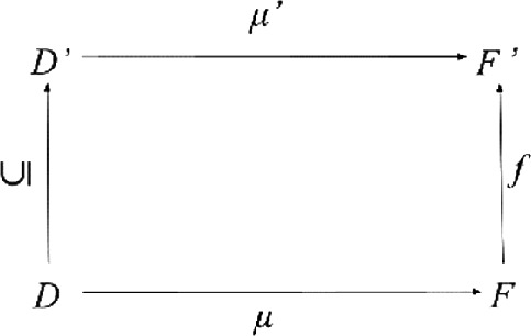
-
(b)
∀x, y ∈ F: x \({\sim}_{\mathcal{F}}\) y → f(x) \({\sim}_{\mathcal{F}\prime}\) f(y).

This definition states that what is indiscernible in the finer representation cannot be discriminated in the coarser representation. The strict version \(\mathcal{F}\)′ is coarser than \(\mathcal{F}\), \(\mathcal{F}\)′> \(\mathcal{F}\), can be defined by the non-strict one:
\(\mathcal{F}\)′> \(\mathcal{F}\) iff \(\mathcal{F}\)′ ≥ \(\mathcal{F}\) and not \(\mathcal{F}\) ≥ \(\mathcal{F}\)′
What we need now is a specification of a relevant set of representations \(\mathcal{H}\). The coarser relation then turns \(\mathcal{H}\) into a preorder. We call such a structure a hierarchy of representations. What is missing to get a partial order from a preorder is the anti-symmetry axiom: from \(\mathcal{F}\) ≥ \(\mathcal{F}\)′ and \(\mathcal{F}\)′ ≥ \(\mathcal{F}\) we cannot conclude that \(\mathcal{F}\) = \(\mathcal{F}\)′. We may have different possibilities to get the same structure of granules. These hierarchies are related to the concept of context (van Rooij 2011).
Definition 9
Hierarchy of representations
A hierarchy \(\mathcal{H}\) is a set of representations such that for any two elements
\(\mathcal{F}\)1/2 = 〈〈F1/2, cl1/2〉, μ1/2, _*1/2, 〈D1/2, _+1/2, _ –1/2, P1/2〉〉 ∈ \(\mathcal{H}\)
we postulate the following constraintsFootnote 35:
-
consistency: ∀p ∈ P1 ∩ P2: (p+1 × p–1) ∩ (p–2 × p+2) = ∅
Elements of p+ and p– cannot change roles in different domains.
-
discriminative power: ∀p ∈ P1 ∩ P2: (p+1 × p–1) ∩ (D2 × D2) ≠ ∅ → p–2 × p+2 ≠ ∅
If a domain contains a discriminating pair of another domain for a shared predicate identifier, it must itself contain a discriminating pair.Footnote 36
Fig. 10 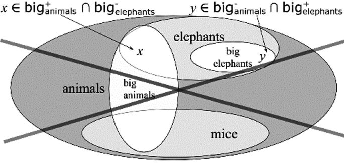
Consistency
Fig. 11 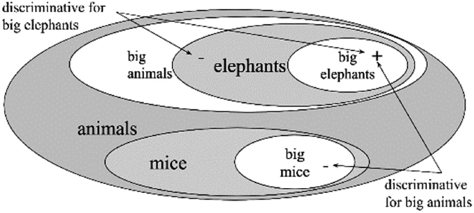
Discriminative power, 1
Fig. 12 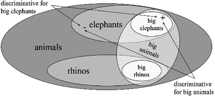
Discriminative power, 2
Fig. 13 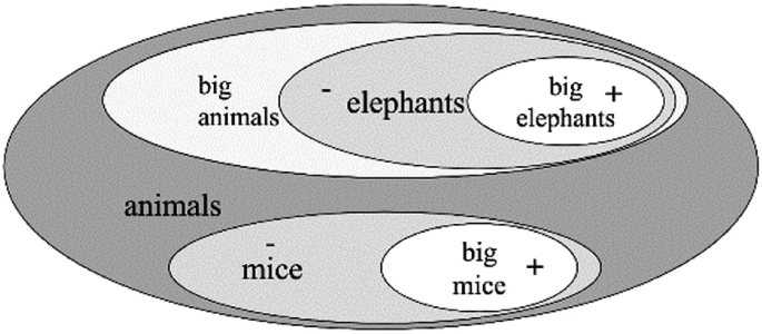
Connectedness
-
connectedness:
∃ \(\mathcal{F}\) = 〈〈F, cl〉, μ, _*, 〈D, _+, _–, P〉〉 ∈ \(\mathcal{H}\): D1 ⊆ D ∧ D2 ⊆ D ∧ P1 ⊆ P ∧ P2 ⊆ P
and there are continues closure preserving functions f1/2: F → F1/2 with μ1/2 = f1/2◦ μ.


For any two domains there is an enclosing domain.
These constraints can be visualized by the Venn diagrams in Fig. 10–13:
-
(a)
the consistency constraint rules out cases like this: if y is a big elephant and x is a small (not big) one, then x cannot be a big animal if y is a small (not big) one (Fig. 10).
-
(b)
discriminative power: If there are big and small elephants there must be big and small animals, too, because animals are different in size: We have big and small elephants which are animals.
-
b1.
If we collect elephants and mice in one animal domain, then a mouse (big or not) is a negative example for big animals. Thus we have a discriminating pair for big animals (Fig. 11).
-
b2.
If we collect only big animals in one animal domain, say elephants, hippos, and rhinoceroses, then any discriminating pair for these species is also discriminative for big animals (Fig. 12).
-
b1.
-
(c)
connectedness: For any two domains there must be a super domain containing both (upward directed) (Fig. 13).
In the remainder of this section we assume that there is a contextually given hierarchy of representations \(\mathcal{H}\). Our approach is non-constructive in the following aspect: We do not construct representations and hierarchies, but instead have systems of constraints which hierarchies must obey. The instantiations must be given by, e.g., the situation of the utterance.
We will now demonstrate how to define a general relation more_sim(a, b, c, d, \(\mathcal{F}\)) based on our similarity relation sim and the preorder on representations. The relation more_sim(a, b, c, d, \(\mathcal{F}\)) is intended to be true if a is more similar to b than c is to d with respect to a representation \(\mathcal{F}\).
Definition 10
More similar
Given a hierarchy \(\mathcal{H}\), a similarity relationFootnote 37 sim, and a representation \(\mathcal{F}\) ∈ \(\mathcal{H}\), we define
more_sim(a, b, c, d, \(\mathcal{F}\)) iff
-
(a)
∃ \(\mathcal{F}\)′ ∈ \(\mathcal{H}\): \(\mathcal{F}\)′ ≥ \(\mathcal{F}\) ∧ sim(a, b, \(\mathcal{F}\)′) ∧ ¬ sim(c, d, \(\mathcal{F}\)′)
-
(b)
∀ \(\mathcal{F}\)′ ∈ \(\mathcal{H}\): \(\mathcal{F}\)′ ≥ \(\mathcal{F}\) → (sim(c, d, \(\mathcal{F}\)′) → sim(a, b, \(\mathcal{F}\)′))
The widely used version more_sim(a, b, c, \(\mathcal{F}\)) in the sense that a is more similar to b than c is similar to b can be defined straightforwardly by:
more_sim(a, b, c, \(\mathcal{F}\)) ≡ more_sim(a, b, c, b, \(\mathcal{F}\))
If a is more similar to b than c to d in a given representation \(\mathcal{F}\) it must be possible to discriminate between c and d. Otherwise, because c and d are maximal similar, a and b cannot be more similar than c and d. If we can discriminate between c and d in \(\mathcal{F}\)′ then we can discriminate between c and d in every finer representation but maybe not in every coarser one. If we can find a representation \(\mathcal{F}\)′ (maybe coarser than \(\mathcal{F}\)), such that we can discriminate between c and d but not between a and b (Definition 10a), we are almost done. It remains to exclude contradictions, that is, representations in which we can discriminate between a and b but not between c and d (this is excluded by Definition 10b).
The diagrams in Fig. 14 and 15 show example hierarchies of representations talking about color and size of objects (each circle stands for a representation). We start with Fig. 14.
Representations which are higher in the hierarchy are coarser than lower ones. On the left branch we introduce a dimension color and a classifier system based on {yellow*, light-blue*, blue*} which can classify colors by convex subsets of a (three-dimensional) color space. On the right branch, we introduce a dimension size with a corresponding classifier system {small*, big*, huge*}. The bottom representation integrates the left branch and the right branch (Definition 9 connectedness). Again, the size dimension need not to be a simple proportional scale. It can itself be a three-dimensional vector space with sub-dimensions length, width, and height.
According to the Definition 10a, the more_sim relation will be inherited from top to bottom along the coarser relation. In the circles, we see the extensions of the corresponding \(\tilde{P}^*\) elements. Next to the circles we see the statements about more_sim which are true in these representations. These statements depend not only on the representation they are attached to, but on the whole upper structure (the filter) of the representation. If we look at the circle at the bottom \(\mathcal{F}\)c+s, we see that we inherit two statements, both from the left branch:
more_sim(y, z, x, \(\mathcal{F}\)c+s) and more_sim(z, y, x, \(\mathcal{F}\)c+s).
From the right branch, we inherit nothing because the classifier system is too weak. Representations may inherit inconsistent information from different paths which rule out some of the statements (by Definition 10b). We can see this when we add more powerful classifiers to the right branch, see Fig. 15.

Hierarchy of representations, Example 1

Hierarchy of representations, Example 2
The two heavily bordered circles (\(\mathcal{F}\)L and \(\mathcal{F}\)R) are alternatives which have different effects on the more fine-grained representations (below). The representation \(\mathcal{F}\)s (circle below \(\mathcal{F}\)L and \(\mathcal{F}\)R) inherits more_sim statements though some are ruled out by the consistency constraint (Definition 10b). In the bottom circle \(\mathcal{F}\)c+s all statements are ruled out by the consistency constraints if both \(\mathcal{F}\)L and \(\mathcal{F}\)R are present in \(\mathcal{H}\). In \(\mathcal{F}\)c+s, more_sim(z, y, x, \(\mathcal{F}\)c+s) would be true (z is more similar to y than x is) according to color because of \(\mathcal{F}\)c″ and Definition 10a. In this case, we cannot discriminate between z and y, but we can discriminate between x and y. According to the existential quantifier in Definition 10a, this is propagated downwards. On the other side, in \(\mathcal{F}\)R we cannot discriminate between x and y. According to the Definition 10b and the universal quantification we should not be able to discriminate between z and y in this representation, but we are. Therefore, we get a contradiction.
Since in a natural language utterance the hierarchy of representations is not explicitly expressed, we can interpret the meaning of an utterance like A is more similar to B than C only as constraint on the relevant hierarchy of representations.
6 Conclusion
We presented a framework introducing a non-metric and qualitative concept of similarity suitable for the interpretation of similarity in natural language.
The basic idea is to “measure” properties of individuals with the help of multi-dimensional attribute spaces representing relevant features of comparison (thus generalizing the idea of degree semantics). In our framework, attribute spaces are complemented by classifiers which are predicates on points in attribute spaces approximating domain predicates; this is what we define as a representation. Individuals count as similar with respect to a particular representation if their values are indistinguishable.
In our framework, the granularity of the similarity relation may vary due to different dimensions of comparison and classifier systems. This leads to sets of representations forming hierarchies of different granularity levels, where the order on representations facilitates a Kleinian style notion of more similar.
This system provides a powerful and flexible tool to capture the meaning of natural language similarity expressions and account for the role of similarity in ad-hoc kind formation as well as equative comparison. Future work will explore its capacity in, e.g., multi-dimensional comparison of adjectival, nominal and verbal properties. The general idea of our approach is to reconstruct comparison in natural language in a qualitative way, with the help of different levels of granularity imposed by constraints on systems of classifiers.
Notes
- 1.
The notion of kinds in linguistics is closely connected to the notion of concepts in psychology (Carlson 2010). Moreover, ad-hoc categories formed by linguistic expressions show core characteristics of concepts (Barsalou 1983). We thus assume that kinds formed ad-hoc by similarity expressions closely correspond to concepts, see Umbach and Stolterfoht (in prep).
- 2.
Starting from Minsky’s frames (Minsky 1975) and feature structures, up to modern approaches based on description logics (for an overview see https://en.wikipedia.org/wiki/Description_logic).
- 3.
For micro-theories in Cyc see, e.g., https://pdfs.semanticscholar.org/4f28/6fdf9280449588b9d3781c9c897da28e0cff.pdf.
- 4.
For an overview of the imagery debate see https://plato.stanford.edu/entries/mental-imagery/.
- 5.
- 6.
There is a long-standing debate about the dichotomy of observables vs. theoretical terms in philosophy, see https://plato.stanford.edu/entries/theoretical-terms-science/. We take a naive view here: observables are functions assigning values to entities in the world which can be determined by ‘simple’ measurements. Examples are temperature, length, width, height, color, position, etc., in contrast to values for energy (which in case of heat, for example, depends on temperature, mass and specific heat of the matter).
- 7.
Our approach is non-constructive since we do not construct representations, but instead have systems of constraints which representations must obey. Bechberger and Kühnberger (this volume) discuss approaches for learning feature space representations by multidimensional scaling. They optimize these representations by using artificial neural networks. From our point of view, they try to learn a feature space F and a measure function μ from similarity and dissimilarity judgments of subjects. In this case, µ maps stimuli (elements of a stimuli domain D) to points in F.
Their approach is restricted such that all dimensions of F have a uniform structure. Essentially F is an euclidean vector space in their approach. There is no canonical interpretation of the dimensions found, and therefore, no link to natural language expressions. In a second step, the goal is to find classifiers which approximate meaningful subclasses of the stimuli space, which may then lead to interpretations of the dimensions. Bechberger and Kühnberger discuss this as a quality measure suited in determining the number of dimensions of F. They generalize the approach to handle unseen stimuli.
- 8.
Classification problems are common in artificial intelligence, where classifiers are trained on huge example sets to be able to classify unseen examples without error. Analogous to our approach, the first step is to find a suitable representation of the real world problems which can be handled by the classification algorithm. Then the example cases have to be translated into this representation in order for the classifier to be able to learn.
- 9.
We may want to restrict computational complexity of classifiers since there should be efficient algorithms for classification. We will pay with accuracy to get easy to classify areas within the attribute space.
- 10.
Open sets are sets without a border. Think of a ball in three-dimensional Euclidean space as something like a tomato: It has a crisp border. If we remove the border by peeling, it is unclear where the tomato ends.
- 11.
In fact, we will often use characteristic functions in place of predicates. In the structures we are interested in, there is an isomorphism between ℘(D) and ΩD. We will not restrict ourselves to a special type of logic (e.g. two-valued classical logic). We stipulate a logical system characterized by a set of truth-values Ω. Ω = {true, false} for classical logic, Ω = [0, 1] for fuzzy logic.
- 12.
We will drop the index D whenever it is clear which domain we are talking about.
- 13.
Positive examples must be in the domain, negative examples may be anywhere. A small mouse is a negative example for ‘big elephant’, but a small elephant is a more informative example.
- 14.
- 15.
Note that ordinal or metric dimensions as common in degree semantics correspond to one-dimensional attribute spaces in our approach.
- 16.
More precisely: p* ◦ μ approximates p.
- 17.
For every p ∈ P there is a p* ∈ P*.
- 18.
This includes all points in the convex closure of the images of the positive exemplars. For the concept of convexity in conceptual structures see Gärdenfors (2000). Intuitively, the convex closure of a subset X of F is the smallest convex subset of F containing X.
- 19.
In most cases, we do not expect to explicitly compute values of the measure function for entities in D. Almost no one will be able to compute the horse power of his car. To learn about the horse power of my car I would look-up the value in the data sheet. When you go to the doctor for a general health check-up the chance that she will take a measure stick to measure your height is very small. It might instead be like this: doctor: “How tall are you?”, patient: “As tall as you.”, doctor: “About 1.75?”, patient: “Think so.” Nevertheless, it should at least in principle be possible to determine the value for a given element in D. It is even possible to use of machine learning technics to learn suitable dimensions and values by analyzing similarity judgments of subjects (see footnote 7).
- 20.
Where ΩF is the set of characteristic functions F → Ω. In addition, we expect that classification functions come with algorithmic methods to compute these functions.
- 21.
There is an interaction between the attribute space F and the measure function μ. While attribute spaces can provide highly structured representations, classifiers can be viewed as attributes with values in Ω. It is possible to hide all the complex structure of a representation in the measure function by using (p1* \(\times\cdots\times\) pn*)◦μ as new measure function and Ωn as attribute space F. Of course that is not the idea of this approach. We will try to use ‘simple’ measure functions and meaningful attribute dimensions.
- 22.
In general, complements of concepts are not necessarily themselves concepts—a non-car is not a proper concept.
- 23.
It has been argued that (3a) and (3b, c) just differ in being one-dimensional as opposed to multi-dimensional, and that even multi-dimensional comparison is scalar. There are, in fact, multi-dimensional adjectives like healthy that allow for comparatives: A is more healthy than B. Sassoon (2013) suggests to interpret comparatives of multi-dimensional adjectives by quantification over dimensions in which the compared entities exceed the standard: A is more healthy than B iff the number of dimensions in which A exceeds the standard is greater than that of B exceeding the standard (for alternatives see the subsection on gradability below).
This approach presupposes, however, that the individual dimensions are scalar, which is not generally the case, consider, e.g., color as a dimension in comparing cars or posture as a dimension in comparing dancing habits. Moreover, even though cars and dancing habits can be compared in equatives, forming comparatives is impossible. This is strong evidence that (3b,c) are genuinely non-scalar.
- 24.
See the quasi exactly implementation of the at-least reading by right closure of classifiers in Sect. 4.
- 25.
Contexts have to be consistent with the order of individuals in the domain.
- 26.
Analogous to thresholds in a single dimension—context-dependent and maybe judge-dependent.
- 27.
The principal filter of x is {q ∈ \(\tilde{P}^*\) | q(x)}.
- 28.
sim′ uses the second argument as point of reference.
- 29.
A metric distance function δ has to comply with (i) minimality: δ(a, b) ≥ δ(a, a) = 0, (ii) symmetry: δ(a, b) = δ(b, a) and (iii) triangle inequality: δ(a, b) + δ(b, c) ≥ δ(a, c).
- 30.
sim′ (Definition 7c) is in fact intransitive due to using the second argument as point of reference.
- 31.
In Tversky’s contrast model a function S takes weighted sums of the feature sets A and B of objects a and b to an interval scale such that sim(a, b) ≤ sim(c, d) iff S(a, b) ≤ S(c, d), where S(a, b) = θf(A ∩ B) – αf(A − B) – βf(B − A), α, β, θ denote weighting functions and f denotes a nonnegative scale.
- 32.
There is also the issue of which features are activated in the first place. In a directional presentation the subject will determine which features are relevant in comparison.
- 33.
If we have a simple interval scale, we can model the at-least reading directly by the order of the attribute values. If we want to model granularity in addition, it becomes more complex since granules may overlap. If the scale is weaker or multiple dimensions are involved, comparison becomes even more complex. Our approach provides a uniform framework for all these cases.
- 34.
Since we have to select the granule first, it is a kind of ‘local’ equivalence class.
- 35.
- 36.
- 37.
We discussed different similarity relations (see Sect. 4). In this definition, we can use any of these.
References
Anderson, C., & Morzycki, M. (2015). Degrees as kinds. NLLT, 33(3).
Barsalou, L. W. (1983). Ad hoc categories. Memory & Cognition, 11(3), 211–222.
Barsalou, L. W. (1992). Frames, concepts, and conceptual fields. In E. Kittay & A. Lehrer (Eds.), Frames, fields, and contrasts. Hillsdale, NJ: Lawrence Erlbaum Associates.
Carlson, G. (1980). Reference to kinds in English. Garland.
Carlson, G. (2010). Generics and concepts. In F. J. Pelletier (Ed.), Kinds, things and stuff (pp. 16–36). Oxford: Oxford University Press.
Carpenter, B. (1992). The logic of typed feature structures. Cambridge Tracts in Theoretical Computer Science, Cambridge University Press.
Gärdenfors, P. (2000). Conceptual spaces. MIT Press.
Gleitman, L., Gleitman, H., Miller, C., & Ostrin, R. (1996). Similar, and similar concepts. Cognition, 58, 321–376.
Greenberg, Y. (2003). Manifestations of genericity. Routledge.
Gust, H., & Umbach, C. (2015). Making use of similarity in referential semantics. In H. Christiansen, I. Stojanovic & G. Papadopoulos (Eds.), Proceedings of the 9th Conference on Modeling and Using Context, Context 2015. LNCS. Springer.
Horn, L. (1992). The said and the unsaid. In B. Chris, & D. David (Eds.), Proceedings of Semantics and Linguistic Theory 2 (pp. 163–192). OSU Working Papers in Linguistics.
Kaplan, D. (1989). Demonstratives. In J. Almog, J. Perry & H. Wittstein (Eds.), Themes from Kaplan (pp. 481–563). Oxford University Press.
Kennedy, C. (1999). Projecting the adjective. Garland Press.
Kennedy, C. (2013). A scalar semantics for scalar readings of number words. In I. Caponigro, & C. Cecchetto (Eds.), From Grammar to Meaning: The Spontaneous Logicality of Language. Cambridge University Press.
Klein, E. (1980). A semantics for positive and comparative adjectives. Linguistics & Philosophy, 4(1), 1–45.
König, E., & Umbach, C. (2018). Demonstratives of manner, of quality and of degree: A neglected subclass. In M. Coniglio, E. Schlachter & T. Veenstra (Eds.), Atypical demonstratives: Syntax, semantics and typology. Berlin, de Gruyter Mouton.
Korte, B., Lovász, L., & Schrader, R. (1991). Greedoids. Springer.
Minsky, M. L. (1975). A framework for representing knowledge. In P. H. Winston (Ed.), The psychology of computer vision. New York.
Nunberg, G. (1993). Indexicality and deixis. Linguistics and Philosophy, 16(1), 1–43.
Nunberg, G. (2004). Indexical descriptions and descriptive indexicals. In M. Reimer & A. Bezuidenhout (Eds.), Descriptions and beyond. Oxford University Press.
Pawlak, Z. (1998). Granularity of knowledge, indiscernibility and rough sets. In Proceedings of the IEEE International Conference on Fuzzy Systems (pp. 106–110).
Prasada, S., & Dillingham, E. M. (2006). Principled and statistical connections in common sense conception. Cognition, 99, 73–112.
Prasada, S., Khemlani, S., Leslie, S.-J., & Glucksberg, S. (2013). Conceptual distinctions amongst generics. Cognition, 126, 405–422.
van Rooij, R. (2011). Implicit versus explicit comparatives. In P. Égré & N. Klinedinst (Eds.), Vagueness and language use (pp. 51–72). Palgrave Studies in Pragmatics, Language and Cognition. Palgrave Macmillan, London.
Sassoon, G. (2013). A typology of multidimensional adjectives. Journal of Semantics, 30, 335–380.
Solt, S. (2016). Multidimensionality, subjectivity and scales: experimental evidence. In E. Castroviejo, L. McNally & G. Sassoon (Eds.), Gradability, scale structure and vagueness: Experimental perspectives. Springer.
Solt, S., & Waldon, B. (2019). Numerals under negation: Empirical findings. Glossa, 4(1), 113.
Tversky, A. (1977). Features of similarity. Psychological Review, 84, 327–352.
Umbach, C., & Gust, H. (2014). Similarity demonstratives. Lingua, 149, 74–93.
Umbach, C., & Gust, H. (in print). Grading similarity. In S. Löbner, T. Gamerschlag, T. Kalenscher, M. Schrenk & H. Zeevat (Eds.), Concepts, frames and cascades in semantics, cognition and ontology. Springer.
Umbach, C., & Stolterfoht, B. (in prep.). Ad-hoc kind formation by similarity.
Acknowledgements
We presented previous versions of this paper at the SFB 991 Kolloquium (Düsseldorf, 2016), the Semantics Colloquium of the Institute of Linguistics (Frankfurt/M, 2017), the ZAS workshop Records, Frames and Attribute Spaces (Berlin, 2018), and the workshop Concepts in Action: Representation, Learning, and Application (Osnabrück, 2018). We would like to thank the colleagues in the audience, and in particular Robin Cooper, Peter Gärdenfors, Wiebke Petersen, Stephanie Solt, Henk Zeevat and Ede Zimmermann for their valuable comments. Finally, we would like to express our gratitude to the editors of this volume for their patience and support. The first author acknowledges financial support by the DFG (UM 100/1-3).
Author information
Authors and Affiliations
Corresponding author
Editor information
Editors and Affiliations
1 Electronic supplementary material
Below is the link to the electronic supplementary material.
Rights and permissions
Open Access This chapter is licensed under the terms of the Creative Commons Attribution 4.0 International License (http://creativecommons.org/licenses/by/4.0/), which permits use, sharing, adaptation, distribution and reproduction in any medium or format, as long as you give appropriate credit to the original author(s) and the source, provide a link to the Creative Commons license and indicate if changes were made.
The images or other third party material in this chapter are included in the chapter's Creative Commons license, unless indicated otherwise in a credit line to the material. If material is not included in the chapter's Creative Commons license and your intended use is not permitted by statutory regulation or exceeds the permitted use, you will need to obtain permission directly from the copyright holder.
Copyright information
© 2021 The Author(s)
About this chapter

Cite this chapter
Gust, H., Umbach, C. (2021). A Qualitative Similarity Framework for the Interpretation of Natural Language Similarity Expressions. In: Bechberger, L., Kühnberger, KU., Liu, M. (eds) Concepts in Action. Language, Cognition, and Mind, vol 9. Springer, Cham. https://doi.org/10.1007/978-3-030-69823-2_4
Download citation
DOI: https://doi.org/10.1007/978-3-030-69823-2_4
Published:
Publisher Name: Springer, Cham
Print ISBN: 978-3-030-69822-5
Online ISBN: 978-3-030-69823-2
eBook Packages: Religion and PhilosophyPhilosophy and Religion (R0)