
Abstract
In this paper, we calculate the vector, axial-vector and tensor form factors of \(P\rightarrow T\) transition within the standard light-front (SLF) and covariant light-front (CLF) quark models (QMs). The self-consistency and Lorentz covariance of CLF QM with two types of correspondence schemes are investigated. The zero-mode effects and the spurious \(\omega \)-dependent contributions to the form factors of \(P\rightarrow T\) transition are analyzed. Employing a self-consistent CLF QM, we present our numerical predictions for the vector, axial-vector and tensor form factors of \(c\rightarrow (q,s)\) (\(q=u,d\)) induced \(D \rightarrow (a_2,K^*_2)\), \(D_s \rightarrow (K^*_2,f'_{2})\), \(\eta _c(1S) \rightarrow (D^*_2,D^*_{s2})\), \( B_c \rightarrow (B^*_2,B^*_{s2})\) transitions and \(b\rightarrow (q,s,c)\) induced \(B \rightarrow (a_2,K^*_2,D^*_2)\), \(B_s \rightarrow (K^*_2,f'_2,D^*_{s2})\), \(B_c \rightarrow (D^*_2,D^*_{s2},\chi _{c2}(1P))\), \(\eta _b(1S) \rightarrow (B^*_2,B^*_{s2})\) transitions. Finally, in order to test the obtained form factors, the semileptonic \(B\rightarrow {\bar{D}}_2^*(2460)\ell ^+\nu _\ell \) (\(\ell =e,\mu \)) and \({\bar{D}}_2^*(2460)\tau ^+\nu _{\tau }\) decays are studied. It is expected that our results for the form factors of \(P\rightarrow T\) transition can be applied further to the relevant phenomenological studies of meson decays.
1 Introduction
In the quark model, mesons are bound states of quark q and antiquark \({\bar{q}}'\), and thus the spin-parity quantum number \(J^P\) of mesons are consequently fixed by the constituent quark pair, for instances \(J^P= 0^-\) for pseudoscalar (P) meson and \(J^P= 2^+\) for p-wave tensor (T) meson. Many tensor mesons have been well established in various processes [1]. Following the flavor SU(3) symmetry, nine possible tensor \((q{\bar{q}}')\) states containing the light u, d, and s quarks, isovector mesons \(a_2(1320)\), isodoulet states \(K^*_2(1430)\) and two isosinglet mesons \(f_2(1270)\), \(f'_2(1525)\) form the \(1^3P_2\) nonet [1]. The known open charm and bottom p-wave tensor states include \(D_{2}^*(2460)\), \(D_{s2}^*(2573)\), \(B_2^*(5747)\) and \(B_{s2}^*(5840)\), the charmonium and bottomonium tensor mesons are \(\chi _{c2}(1P )\) and \(\chi _{b2}(1P )\), respectively.
The B and D meson decays induced by heavy-to-light transition provide a fertile ground for testing the Standard Model (SM) and searching for new physics (NP). Some discrepancies between the experimental data and the SM predictions have been found, for instance, the SM predictions for \(R_{D^{(*)}}\) deviate from data by more than \(3\sigma \) errors [2]. If these tensions are confirmed by the forthcoming experiments, the discrepancies should also be seen in B transitions to tensor mesons in addition to B decays to pseudoscalar or vector mesons. The decay modes involving tensor final states are of great interest because the tensor meson has additional polarization states compared with the (pseudo)scalar and (axial)vector mesons and thus the relevant decays may have more kinematical quantities related to the underlying helicity structure. Some theoretical studies on these decays have been made in, for instance, Refs. [3,4,5,6,7,8,9,10,11,12,13,14,15,16,17,18,19,20,21]. In the calculation of the amplitudes of semi-leptonic, non-leptonic and radiative B and D meson decays, the form factors serve as the basic and important input parameters.
There are many approaches for evaluating the form factors, for instance, Wirbel-Stech-Bauer model [22], lattice QCD (LQCD) [23], perturbative QCD (PQCD) with some nonperturbative inputs [24, 25], QCD sum rules (QCD SR) [26, 27], light-front quark models (LF QMs) [28,29,30,31,32,33,34], etc. Some \(B\rightarrow T\) transition form factors have be evaluated by employing the light-cone sum rules (LCSRs) approach [35,36,37], QCD SR [38], the large energy effective theory (LEET) [39, 40] and PQCD approach [41]. In this paper, we will evaluate the form factors of \(c\rightarrow (q,s)\) (\(q=u,d\)) induced \(D \rightarrow (a_2,K^*_2)\), \(D_s \rightarrow (K^*_2,f'_{2})\), \(\eta _c(1S) \rightarrow (D^*_2,D^*_{s2})\), \( B_c \rightarrow (B^*_2,B^*_{s2})\) transitions and \(b\rightarrow (q,s,c)\) induced \(B \rightarrow (a_2,K^*_2,D^*_2)\), \(B_s \rightarrow (K^*_2,f'_2,D^*_{s2})\), \(B_c \rightarrow (D^*_2,D^*_{s2},\chi _{c2}(1P))\), \(\eta _b(1S) \rightarrow (B^*_2,B^*_{s2})\) transitions within the standard and the covariant light-front quark models.
The standard light-front quark model (SLF QM) [28,29,30,31] is based on the LF formalism [42] and LF quantization of QCD [43], and provides a conceptually simple and phenomenologically feasible framework for evaluating nonperturbative quantities. However, in this approach, the matrix element lacks manifest Lorentz covariance and the zero-mode contributions can not be determined explicitly. Therefore, a basically different technique is developed by Jaus to deal with the covariance and the zero-mode problems with the help of a manifestly covariant Bethe-Saltpeter (BS) approach as a guide to the calculation [33]. In such a covariant light-front quark model (CLF QM), the zero-mode contributions can be well determined, and the matrix element is expected to be covariant because the \(\omega \)-dependent spurious contributions, where \(\omega \) is the light-like four-vector used to define light-front by \(\omega \cdot x=0\), can be eliminated by the inclusion of zero-mode contributions [33].
Unfortunately, the covariance of matrix element in fact can not be fully recovered in such traditional CLF QM because there are still some residual \(\omega \)-dependent spurious contributions associated with B functions [33, 44]. In addition, the traditional CLF QM suffers from a self-consistence problem for a long time, for instance, it has been found that the CLF results for \(f_V\) obtained respectively via longitudinal (\(\lambda =0\)) and transverse (\(\lambda =\pm \)) polarization states are inconsistent with each other [45], \([f_V]_{\mathrm{CLF}}^{\lambda =0}\ne [f_V]_{\mathrm{CLF}}^{\lambda =\pm }\), because the former receives an additional contribution characterized by the \(B_1^{(2)}\) function. Another self-consistence problem has also been found in Ref. [46].
In order to deal with the self-consistence problem, Choi and Ji present a modified correspondence scheme between the covariant BS approach and the LF approach (named as type-II scheme) [47], which requires an additional \(M\rightarrow M_0\) replacement relative to the traditional type-I correspondence scheme. By using such improved self-consistent CLF QM, one can obtain the self-consistent results [47], and moreover, the covariance of matrix element can be fully recovered [44, 46, 48, 49]. In this paper, we would like to further test the self-consistence and covariance of the self-consistent CLF QM via the form factors of \(P\rightarrow T\) transition.
Our paper is organized as follows. In Sect. 2, the SLF and the CLF QMs are review briefly, and then our theoretical results for the vector, axial-vector and tensor form factors of \(P\rightarrow T \) transition are presented. In Sect. 3, the self-consistency and covariance of CLF results are discussed, and the zero-mode and the valence contributions are analyzed. After that, our numerical results for the \(c\rightarrow (q,s)\) (\(q=u,d\)) induced \(D\rightarrow (a_2,K^*_2)\), \(D_s\rightarrow (K^*_2, f'_2)\), \(\eta _c(1S)\rightarrow (D^*_2,D^*_{s2})\), \(B_c\rightarrow (B^*_2,B^*_{s2} )\) transitions and the \(b\rightarrow (q,s,c)\) induced \(B\rightarrow (a_2,K^*_2, D^*_2), B_s\rightarrow (K^*_2, f'_2, D^*_{s2}), B_c\rightarrow (D^*_2, D^*_{s2}, X_{c2}(1P))\), \(\eta _b(1S)\rightarrow (B^*_2,B^*_{s2})\) transitions are given. Finally, a summary is given in Sect. 4.
2 Theoretical framework and results
2.1 Definitions of form factors
The matrix elements of \(P\rightarrow T\) transition with vector, axial-vector and tensor currents are commonly factorized in terms of form factors as [3, 50]
where, \( \varepsilon _{0123}=-1\), \(P=p'+p''\), \(q=p'-p''\), \(e^{*\nu }\equiv \frac{\epsilon ^{*\mu \nu }\cdot p'_{\mu }}{M'}\), \(M^{'('')}\) is the mass of initial (final) state, \(\epsilon ^{\mu \nu }\) is the polarization tensor of tensor meson and satisfies \(\epsilon ^{\mu \nu } p''_{\nu }=0\). The polarization tensors \(\epsilon ^{\mu \nu }(\lambda )\) with \(\lambda \) helicity (\(\lambda =0,\pm 1,\pm 2\) ) can be constructed in terms of the polarization vectors of vector state \(\epsilon ^{\mu }{(\lambda ')}\), and explicitly written as
where,
Using the identity \(2\sigma ^{\mu \nu } \gamma _5=i \varepsilon ^{\mu \nu \alpha \beta }\sigma _{\alpha \beta } \), one can rewrite the definition of tensor form factors \(T_{1,2,3}\), Eq. (3), as
which is much more convenient for extracting the form factors within the SLF QM.
2.2 Theoretical results in the SLF QM
In order to clarify the convention and notation used in this paper, we would like to review briefly the framework of SLF QM. One may refer to, for instance, Refs. [28,29,30,31] for details.
The main work of LF approach is to evaluate the current matrix element,
which will be further used to extract the form factors. The meson bound-state (\(q_1{{\bar{q}}}_2\)) with total momentum p and spin J can be written as
where \(k_1\) and \(k_2\) are the on-mass-shell light-front momenta and can be written in terms of the internal relative momentum variables \((x,{{\mathbf {k}}_{\bot }})\) as
with \({\bar{x}}\equiv 1-x\).
The momentum-space wavefunction (WF) for a \(^{2S+1}L_J\) meson, \(\Psi _{LS}^{JJ_z}({k}_1,h_1,{k}_2,h_2)\), in Eq. (10) satisfies the normalization condition and can be expressed as
where, \(\psi (x,{\mathbf {k}}_{\bot })\) is the radial WF and responsible for describing the momentum distribution of the constituent quarks in the bound-state; \(S_{h_1,h_2}(x,{\mathbf {k}}_{\bot })\) is the spin-orbital WF and responsible for constructing a state of definite spin \((S,S_z)\) out of the LF helicity \((h_1,h_2)\) eigenstates. For the former, we adopt the Gaussian type WF
where, \(k_z\) is the relative momentum in z-direction, \(k_z=(x-\frac{1}{2})M_0+\frac{m_2^2-m_1^2}{2 M_0}\), with the invariant mass \(M_0^2=\frac{m_1^2+{\mathbf {k}}_{\bot }^2}{x}+\frac{m_2^2+{\mathbf {k}}_{\bot }^2}{{\bar{x}}}\). The spin-orbital WF, \(S_{h_1,h_2}(x,{\mathbf {k}}_{\bot }) \), can be obtained by the interaction-independent Melosh transformation. It is convenient to use its covariant form, which can be further reduced by using the equation of motion on spinors and finally written as [31, 45]
where, \({\hat{M}}_0^2=M_0^2-(m_1-m_2)^2\). For P and T mesons, the vertices \(\Gamma '\) are written as
where \({\hat{\epsilon }}^{\mu \nu }=\epsilon ^{\mu \nu }(M\rightarrow M_0)\).
Using the formulae given above, the matrix element of \(M'\rightarrow M''\) transition can be written as
where \(S'^{(\prime \prime )}\) and \(\psi '^{(\prime \prime )}\) are the WFs of initial (final) state; \(C_{h''_1,h'_1}(x,{\mathbf {k}}_{\bot }',{\mathbf {k}}_{\bot }'') \equiv {\bar{u}}_{h''_1}(x,{\mathbf {k}}_{\bot }'') \Gamma u_{h'_1}(x,{\mathbf {k}}_{\bot }')\) with \(\Gamma \) given by Eq. (9) for \(P\rightarrow T\) transition. In the further calculation, it is covariant to use the Drell-Yan-West frame, \(q^+=0\), and take a Lorentz frame, \({\mathbf {p}}_{\bot }'=0\). In this frame, the momenta of constituent quarks in initial and final states are written as
where \({\mathbf {p}}_{\bot }''={\mathbf {p}}_{\bot }'-{\mathbf {q}}_{\bot }=-{\mathbf {q}}_{\bot }\) and \({\mathbf {k}}_{\bot }''={\mathbf {k}}_{\bot }'-{\bar{x}}{\mathbf {q}}_{\bot }\).
In the SLF QM, in order to extract the form factors of \(P\rightarrow T\) transition defined by Eqs. (1-3), one has to take explicit values of \(\mu \) and/or \(\lambda \). In this work, we take the following strategyFootnote 1:
-
For the vector form factor V, we take \(\lambda ''=+2\) and multiply both sides of Eq. (1) by \( \epsilon ^{\mu }\).
-
For the axial-vector form factors, we take \(\mu =+\), and then use \({{\mathcal {B}}}_{\mathrm{SLF}}^+\) with \(\lambda ''=+2\) and \(+1\) to extract \(A_{2}\) and \(A_{1}\), respectively; we take \(\lambda ''=+2\), and multiply both sides of Eq. (2) by \(q^{\mu }\) to extract \(A_{0}\).
-
For the tensor form factors, we take \(\lambda ''=+2\), and multiply both sides of Eq. (8) by \( \epsilon ^{\mu }q^{\nu }\), \( \epsilon ^{\mu }P^{\nu }\) and \( \epsilon ^{\mu } \epsilon ^{*\nu }\) to extract \(T_1\), \(T_2\) and \(T_3\), respectively.
After some derivations and simplifications, we finally obtain the SLF results for the form factors of \(P\rightarrow T\) transition written as
where, the integrands are
2.3 Theoretical results in the CLF QM
In order to treat the complete Lorentz covariance of matrix elements and investigate the effect of zero-mode contribution, a theoretical framework of CLF approach is developed by Jaus with the help of a manifestly covariant BS approach as a guide to the calculation. One may refer to Refs. [33, 45, 51] for detail. In the CLF QM, the matrix element is obtained by calculating the Feynman diagram shown by Fig. 1. For the \(P\rightarrow T\) transition, the matrix element can be expressed as
where \(\mathrm{d}^4 k_1'=\frac{1}{2} \mathrm{d}k_1'^- \mathrm{d}k_1'^+ \mathrm{d}^2 {\mathbf {k}}_{\bot }'\), the denominators \(N_{1}^{(\prime ,\prime \prime )}=k_{1}^{(\prime ,\prime \prime )2}-m_1^{(\prime ,\prime \prime )2}+i\varepsilon \) and \(N_{2}=k_{2}^{2}-m_2^{2}+i\varepsilon \) come from the fermion propagators, \(H_{P, T}\) are vertex functions, and \(\epsilon \) is the polarization tensor of tensor meson. The trace term \(S_{{\mathcal {B}}}\) is associated with the fermion loop and is written as
where \(\Gamma _{P,T}\) are the vertex operators written as [45]
As has been stressed in Ref. [33], the covariant calculation and the calculation of the light-front formalism give identical results at the one-loop level if the vertex functions \(H_{P, T}\) are analytic in the upper complex \(k_1'^-\) plane. By closing the contour in the upper complex \(k_1'^-\) plane and assuming that \(H_{P, T}\) are analytic within the contour, the integration picks up a residue at \(k_2^2={\hat{k}}_2^2=m_2^2\) corresponding to putting the spectator antiquark on its mass-shell. After integrating the minus component of loop momentum, the covariant calculation becomes the LF one. Such manipulation ask for the following replacements [33, 45]
and
where the LF form of vertex function, \(h_{P(T)}\), is given by
The Eq. (32) shows the correspondence between manifestly covariant and LF approaches [33, 45], the correspondence between \(\chi \) and h can be clearly derived by matching the CLF expressions to the SLF ones via some zero-mode independent quantities [33, 45]. However, the validity of the correspondence for the D factor appearing in the vertex operator cannot been clarified explicitly [47]. In fact, the traditional type-I correspondence may give self-contradictory results for some quantities. An obvious example is \(f_{V}\) noted by the authors of Ref. [45]. In order to get self-consistent results for \(f_{V}\), a much more generalized correspondence scheme is proposed [47],
Within this updated self-consistent scheme, the CLF QM can give a self-consistent result for \(f_{V,A}\) and form factors of \(P\rightarrow (V,A)\) and \(V'\rightarrow V''\) transitions [44, 47,48,49], while the self-consistency of the form factors of \(P\rightarrow T\) transition remains to be tested.
Using above formulas and integrating out \(k_1'^-\), the matrix element, Eq. (27), can be reduced to the LF form
However, the matrix element obtained in this way contains spurious \(\omega ^\mu \)-dependent contributions, which violate the covariance of matrix element. It should be noted that the contribution of the zero-mode from the \(k_1'^+=0\) is not taken into account in the contour integration. It is interesting that the spurious \(\omega ^\mu \)-dependent terms in \(\hat{{{\mathcal {B}}}}\) can be eliminated by the zero-mode contributions [33]. The inclusion of zero-mode contributions in practice amount to the following replacements
where A and B functions are given by
The \(\omega \)-dependent terms associated with the C functions are not shown because they can be eliminated exactly by the inclusion of the zero-mode contributions [33]. However, there are still some residual \(\omega \)-dependences associated with the B functions, which are irrelevant zero-mode contribution [33], and possibly result in the inconsistence and covariance problems [44, 47,48,49].
Using the formulae given above, one can obtain CLF results for the matrix elements of \(P\rightarrow T\) transition, \({{\mathcal {B}}}_{\mathrm{CLF}}^\mu \). Then, matching obtained \({{\mathcal {B}}}_{\mathrm{CLF}}^\mu (\Gamma = \gamma _\mu )\) , \({{\mathcal {B}}}_{\mathrm{CLF}}^\mu (\Gamma = \gamma _\mu \gamma _5)\) and \({{\mathcal {B}}}_{\mathrm{CLF}}^\mu (\Gamma =\sigma _{\mu \nu }(1+ \gamma _5)q^\nu )\) to the definitions of form factors given by Eqs. (1-3), the CLF results for the form factors of \(P\rightarrow T\) transition can be extracted directly. They can be written as
where the integrands are
The CLF results given above are independent of \(\mu \) and \(\lambda \), which implies that the CLF contributions are irrelevant to the self-consistence and covariance problems. This is a significant advantage of CLF QM compared the SLF QM. However, it should be noted that the contributions associated with B functions are not included in above formulae. These contributions may result in the self-consistence and covariance problems of CLF QM except they are equal to zero numerically, and will be analyzed in the next section.
In our following discussions, we also need the valence contributions, which can be obtained by assuming \(k_2^+\ne 0\) (or \(p^+\ne 0\)). This assumption ensures the pole of \(N_2\) is safely located in the contour of \(k_1'^-\) integral ( the pole of \(N_2\) is finite) and implies that the zero-mode contributions are not taken into account. At this moment, the replacements for \({\hat{k}}_1'^{\mu }\) given above have to be disregarded. Instead, one just need to directly use the on-mass-shell condition of spectator antiquark, \(k_2^2=m_2^2\), and the conservation of four-momentum at each vertex. The valence contributions to the form factors can also be expressed as Eq. (50) with the integrands written as
3 Numerical results and discussion
With the theoretical results given above and the values of input parameters collected in appendix A, we then present our numerical results and discussions in this section. As has been mentioned in the last section, the contributions associated with B functions are not included in the CLF results, Eqs. (51-57). These contributions to the matrix elements of \(P \rightarrow T\) transition can be written as
where, the integrands are
After extracting their contributions to the form factors, \([{{\mathcal {F}}}]^{\mathrm{B}}\), one can obtain the full result of form factor in the CLF QM, which can be expressed as
Based on these results, we have following discussions and findings:
-
Here, we take \(\mathcal{\widetilde{B}}_{\mathrm{B}}(\Gamma =\sigma _{\mu \nu } \gamma _5q^\nu )\) given by Eq. (69) as an example. From this equation, it can be found that the third term is proportional to \(\omega _\mu \). This spurious \(\omega _\mu \)-dependent contribution corresponds to an unphysical form factor and may violate the covariance of matrix element if it is non-zero. The other terms would present contributions to the tensor form factors, \(T_2\) and \(T_3\). For convenience of discussion, we take \(T_3\) as an example, which could receive the contribution from the second term written as
$$\begin{aligned} {\widetilde{ T}_3}^{\mathrm{B}}&=\frac{2(M'^2-M''^2)}{ e^{*}\cdot q}\,\frac{\epsilon ^{\lambda \delta *}q_\lambda \omega _\delta }{\omega \cdot P}\nonumber \\&\quad \bigg \{B^{(2)}_1 \left[ 3+\frac{4(m^{\prime \prime }_1+2m_2-2m^{\prime \prime }_1)}{D_{T,\mathrm{con}}}\right] \nonumber \\&\quad +{4B^{(3)}_1}\left( 1+\frac{m^{\prime }_1-m''_1-2m_2}{D_{T,\mathrm{con}}}\right) \nonumber \\&\quad +\frac{8(m^{\prime }_1-m_2){B^{(3)}_2}}{D_{T,\mathrm{con}}} \bigg \}\,, \end{aligned}$$(71)which is obviously dependent on the choice of \(\lambda ''\). For different values of \(\lambda ''\), \({\widetilde{ T}_3}^{\mathrm{B}}\) can be explicitly written as
$$\begin{aligned} { \widetilde{T}_3}^{\mathrm{B}}=\left\{ \begin{array}{lr} \frac{2M'(M'^2-M''^2)(M'^2-M''^2+q_\bot ^2)}{(M'^2-M''^2)^2+2(M'^2-2M''^2){ \mathbf{q}}_\bot ^2+{ \mathbf{q}}_\bot ^4}\\ \bigg \{B^{(2)}_1 \left[ 3+\frac{4(m^{\prime \prime }_1+2m_2-2m^{\prime }_1)}{D_{T,\mathrm{con}}}\right] \\ +{4B^{(3)}_1}\left( 1+\frac{m^{\prime }_1-m''_1-2m_2}{D_{T,\mathrm{con}}}\right) \\ +{B^{(3)}_2}\frac{8(m^{\prime }_1-m_2)}{D_{T,\mathrm{con}}} \bigg \}\,, &{}\lambda ''=0 \\ \frac{M'(M'^2-M''^2)}{M'^2-M''^2+q_\bot ^2}\\ \bigg \{B^{(2)}_1 \left[ 3+\frac{4(m^{\prime \prime }_1+2m_2-2m^{\prime }_1)}{D_{T,\mathrm{con}}}\right] \\ +{4B^{(3)}_1}\left( 1+\frac{m^{\prime }_1-m''_1-2m_2}{D_{T,\mathrm{con}}}\right) \\ +{B^{(3)}_2}\frac{8(m^{\prime }_1-m_2)}{D_{T,\mathrm{con}}} \bigg \}\,, &{}\lambda ''=\pm 1 \\ 0\,. &{}\lambda ''=\pm 2 \\ \end{array} \right. \end{aligned}$$(72)Fig. 1 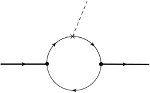
The Feynman diagram for the matrix element within the CLF QM
Table 1 Numerical results of form factor \(T_{3}(\mathbf{{q}}_\perp ^2)\) at \(\mathbf{q}_{\bot }^2=(0,1,4,9) \,\mathrm{GeV^2}\) for \(B_c\rightarrow D^*_2\) transition Further considering the fact that \([{{\mathcal {F}}}]^{\mathrm{CLF}}\) is independent of \(\lambda ''\), it is clearly seen that \(T_3\) possibly suffers from a self-consistence problem (i.e. \([T_{3}]^{\mathrm{full}}_{\lambda =0}\ne [T_{3}]^{\mathrm{full}}_{\lambda =\pm 1}\ne [T_{3}]^{\mathrm{full}}_{\lambda =\pm 2}\)) caused by the B function contributions in the CLF QM. Comparing with the other transitions, the \(P \rightarrow T\) transition is associated with much more B functions, and thus presents a tougher challenge to the CLF QM.
-
In order to clearly show the possible self-consistence problem caused by B functions within type-I and type-II schemes, we define the contributions of B functions \(\Delta _{\mathrm{B}}(x)\) as
$$\begin{aligned} \Delta _{\mathrm{B}}(x) \equiv \frac{\mathrm{d}[{{\mathcal {F}}}^{\mathrm{B}}]_{\lambda ''}}{ \mathrm{d}x}\,, \end{aligned}$$(73)which is equal to \(N_c\int \frac{\mathrm{d}^2\mathbf{k'_\bot }}{2(2\pi )^3}\frac{\chi _P'\chi _T''}{{{\bar{x}}}} {{\widetilde{T}}}^{\mathrm{B}}_{3}\) for the case of \(T_3\). Taking \(D\rightarrow K^*_2\) and \(B_c\rightarrow D^*_2\) transitions as examples, the dependence of \(\Delta _{\mathrm{B}}(x)\) on x are shown in Fig. 1. It can be seen that the self-consistence is violated within the type-I scheme, but it can be satisfied within the type-II scheme due to \(\int _0^1\mathrm{d}x\,[\Delta _{\mathrm{B}}]_{T_3}(x)=0\) for any values of \(\lambda ''\).
In order to further confirm such finding, we list the numerical results of \([T_{3}]^{\mathrm{full}}\) for \(B_c\rightarrow D^*_2 \) transition at \({ \mathbf{q}}_\bot ^2=(0,1,4,9)\,\mathrm{GeV^2}\) with \(\lambda ''=(0,\pm 1,\pm 2)\) in Table 1, in which the SLF, valence and CLF results are also given for comparison. From these numerical results, it is found that \([T_{3}]^{\mathrm{full}}_{\lambda =0}\ne [T_{3}]^{\mathrm{full}}_{\lambda =\pm 1}\ne [T_{3}]^{\mathrm{full}}_{\lambda =\pm 2}\) within the traditional type-I scheme, while
$$\begin{aligned}{}[T_{3}]^{\mathrm{full}}_{\lambda =0}\doteq [T_{3}]^{\mathrm{full}}_{\lambda =\pm 1}\doteq [T_{3}]^{\mathrm{full}}_{\lambda =\pm 2}\,, \qquad { (\text {type-II})} \end{aligned}$$(74)which confirms again that the contribution associated with B functions vanishes numerically within the type-II scheme, even though it exists formally in the expression of form factor given by Eq. (70). In addition, one can also find from Table 1 that the SLF results are also consistent with the CLF ones, \([T_{3}]^{\mathrm{full}}\dot{=}[T_{3}]^{\mathrm{SLF}}\), in type-II scheme. These results confirm again the finding obtained from Fig. 1. Moreover, we have checked the contributions of B functions to the other form factors, and obtain the same conclusion. Therefore, it can be concluded that the CLF results for the form factors of \(P\rightarrow T\) transitions have a self-consistence problem caused by B function contributions within the type-I scheme, but the type-II scheme can give self-consistent results.
-
Besides of the self-consistence, the contributions of B functions also possibly result in a covariance problem because some terms in \(\mathcal{\widetilde{B}}_\mu \) are associated with \(\omega _{\mu }\). Taking the third term in \(\mathcal{\widetilde{B}}_{\mathrm{B}}(\Gamma =\sigma _{\mu \nu } \gamma _5q^\nu )\) given by Eq. (69) as an example, this spurious \(\omega _\mu \)-dependent contribution corresponds to an unphysical form factor and would violate the covariance of matrix element except it vanishes numerically. Similar to the case of \([T_{3}]^{\mathrm{B}}\) discussed above, it is found that this spurious \(\omega _\mu \)-dependent contribution is (non)zero within the type-II (I) scheme, which implies that the Lorentz covariance of \({{\mathcal {B}}}^\mu \) is violated within the type-I correspondence scheme, but such problem can be avoided by employing the type-II scheme.
-
As has been mentioned above, the spurious \(\omega _\mu \)-dependent contributions associated with C functions can be canceled by the zero-mode contributions [33]. The residual zero-mode contributions to form factors can be obtained via \([{{\mathcal {F}}}]^{\mathrm{CLF}}=[{{\mathcal {F}}}]^{\mathrm{val.}}+[{{\mathcal {F}}}]^{\mathrm{z.m.}}\). In order to clearly show the effect of zero-mode contribution, we take \(T_{3}^{B\rightarrow K^*_2\,,D\rightarrow K^*_2}\) as examples and plot the dependence of \(\mathrm{d}[{{\mathcal {F}}}]^{\mathrm{z.m.}}/\mathrm{d}x\) on x in Fig. 2. It can be found that zero-mode presents nonzero contributions within the traditional type-I correspondence scheme; while, these contributions, although existing formally, vanish numerically in the type-II correspondence scheme, i.e., \([T_{3}(q^2)]_{\mathrm{z.m.}}\dot{=} 0\) (type-II), because the contribution with small x and the one with large x cancel each other out exactly at each \({{ \mathbf{q}}_\bot ^2}\) point. This can also be found from the numerical results given by Table 1.


The dependences of \([\Delta _B]_{T_{3}}(x)\) on x for \(D\rightarrow K^*_2\) transition at \(\mathbf{q}_{\bot }^2=(0,0.2)\,\mathrm{GeV^2}\) and for \(B_c\rightarrow D^*_2\) transition at \(\mathbf{q}_{\bot }^2=(0,9)\,\mathrm{GeV^2}\)

The dependences of \(\mathrm{d}[{ T_3}]^{\mathrm{z.m.}}/\mathrm{d}x\) on x for \(D\rightarrow K^*_2\) transition at \(\mathbf{q}_{\bot }^2=(0,0.2)\,\mathrm{GeV^2}\) and for \(B_c\rightarrow D^*_2\) transition at \(\mathbf{q}_{\bot }^2=(0,9)\,\mathrm{GeV^2}\)
The tensor form factors of \(P \rightarrow T\) transition have also been calculated by Cheng and Chua (CC) [50] within the traditional CLF QM, their results are given in appendix B. The contributions associated with B functions are not considered in their calculation. Besides, comparing CC’s results with ours, it is found that they are the same for \(T_1\), but are obviously different for \(T_2\) and \(T_3\) in form. In addition, it has been checked that their numerical results for \(T_2\) and \(T_3\) are different either within type-I scheme. After checking our and CC’s calculations, we find another inconsistent problem caused by the different way for dealing with the trace term \(S^{P\rightarrow T}_{\mu \nu \lambda \delta }\) related to the matrix element \({{\mathcal {B}}}^{P\rightarrow T}_{\mathrm{CLF}}[\Gamma =\sigma _{\mu \nu }\gamma _5]\). To clarify the origin of this inconsistent problem, we take the term \(2ig_{\nu \lambda }g_{\alpha \mu }g_{\beta \sigma }(P+q)^{\beta }k'^{\sigma }_1k'^{\alpha }_1k'_{1\delta }\) appeared in \(S^{P\rightarrow T}_{\mu \nu \lambda \delta }\) as an example. As has been mentioned in the last section, some replacements are needed to take the zero-mode contribution into account after integrating out \(k'^-_1\). In the CC’s calculation, the replacement for \({\hat{k}}'^{\sigma }_1{\hat{k}}'^{\alpha }_1{\hat{k}}'^{\delta }_1\) is used directly though \(\sigma \) is a dummy indices, i.e.,
In our calculation, we employ the standard procedure of CLF calculation, and obtain
Comparing Eq. (76) with Eq. (75), one can easily find that CC’s result is different from ours because different replacements are needed. As a result, our and CC’s results for \(T_{2,3}\) are different in form.
In order to clearly show the divergence between CC’s and our results, we define the difference
where \({{\mathcal {F}}}=T_{2,3}\). Then, taking \(D\rightarrow K^*_2\) and \(B_c \rightarrow D^*_2\) as examples, the dependences of \(\Delta _{T_{2,3}}^{\mathrm{CLF}}(x,{ \mathbf{q}}_\bot ^2)\) on x in type-I and -II schemes are shown in Fig. 3. It can be easily seen from Fig. 3 that our and CC’s numerical results for \(T^{\mathrm{CLF}}_{2,3}\) are inconsistent within the type-I scheme; however, such inconsistence problem vanishes in the type-II scheme due to \(\int ^1_0 dx \Delta _{{ T}_{2,3}}^{\mathrm{CLF}}(x)\dot{=}0 \).
From above discussions, one can conclude that the CLF QM with type-II corresponding scheme can make sure the Lorentz covariance of matrix elements and give self-consistent results for the form factors. Using the values of input parameters collected in appendix A and employing the self-consistent type-II scheme, we then present our numerical predictions for the form factors of \(c\rightarrow (q,s)\) (\(q=u,d\)) induced \(D\rightarrow (a_2,K^*_2)\), \(D_s\rightarrow (K^*_2, f'_2)\), \(\eta _c(1S)\rightarrow (D^*_2,D^*_{s2})\), \(B_c\rightarrow (B^*_2,B^*_{s2} )\) transitions and \(b\rightarrow (q,s,c)\) induced \(B\rightarrow (a_2,K^*_2, D^*_2), B_s\rightarrow (K^*_2, f'_2, D^*_{s2}), B_c\rightarrow (D^*_2, D^*_{s2}, X_{c2}(1P))\), \(\eta _b(1S)\rightarrow (B^*_2,B^*_{s2})\) transitions.
It should be noted that the CLF calculation is made in the \(q^+=0\) frame, which implies that the form factors are known only for space-like momentum transfer, \(q^2=-{\mathbf {q}}_\bot ^2\leqslant 0\), and the results in the time-like region need an additional \(q^2\) extrapolation. For the phenomenological applications, we adopt the BCL version of the z-series expansion [52] in the form adopted in Refs. [53, 54],
where, \(z(q^2, t_0)=\frac{\sqrt{t_+-q^2}-\sqrt{t_+-t_0}}{\sqrt{t_+-q^2}+\sqrt{t_+-t_0}}\), \(t_+=(M'+ M'')^2\), \(t_0=(M'+ M'')(\sqrt{M'}-\sqrt{M''})^2\). For the masses of resonances collected in Table 2, we take the values given by PDG [1] and lattice QCD [55, 56]. In the practice, we will truncate the expansion at \(N=1\). The parameter \(b_k\) will be obtained by fitting to the results computed directly by CLF QMs.
Using the parameterization scheme given by Eq. (78), we present our numerical results of \({{\mathcal {F}}}(0)\) and \(b_1\) for the \(c\rightarrow (q,s)\) (\(q=u,d\)) induced \(D\rightarrow (a_2,K^*_2)\), \(D_s\rightarrow (K^*_2, f'_2)\), \(\eta _c(1S)\rightarrow (D^*_2,D^*_{s2})\), \(B_c\rightarrow (B^*_2,B^*_{s2} )\) transitions and the \(b\rightarrow (q,s,c)\) induced \(B\rightarrow (a_2,K^*_2, D^*_2), B_s\rightarrow (K^*_2, f'_2, D^*_{s2}), B_c\rightarrow (D^*_2, D^*_{s2}, X_{c2}(1P))\), \(\eta _b(1S)\rightarrow (B^*_2,B^*_{s2})\) transitions in Tables 3 and 4, respectively. The \(q^2\) dependence of form factors are shown in Figs. 4 and 5. Some remarks on these results are given in order.

The dependences of \(\Delta _{T_{2,3}}^{\mathrm{CLF}}\) on x for \(D\rightarrow K^*_2\) transition at \(\mathbf{q}_{\bot }^2=(0,0.2)\,\mathrm{GeV^2}\) and for \(B_c\rightarrow D^*_2\) transition at \(\mathbf{q}_{\bot }^2=(0,9)\,\mathrm{GeV^2}\)

The \(q^2\) dependence of form factors of \(c\rightarrow (q,s)\) induced \(D \rightarrow (a_2,K^*_2)\), \(D_s \rightarrow (K^*_2,f'_{2})\), \(\eta _c(1S) \rightarrow (D^*_2,D^*_{s2})\), \( B_c \rightarrow (B^*_2,B^*_{s2})\) transitions

The \(q^2\) dependence of form factors of \(b\rightarrow (q,s,c)\) induced \(B \rightarrow (a_2,K^*_2,D^*_2)\), \(B_s \rightarrow (K^*_2,f'_2,D^*_{s2})\), \(B_c \rightarrow (D^*_2,D^*_{s2},\chi _{c2}(1P))\), \(\eta _b(1S) \rightarrow (B^*_2,B^*_{s2})\) transitions

The \(q^2\)-dependence of form factors of \(B\rightarrow D^*_2\) and \(B\rightarrow K^*_2\) transitions within the truncation-schemes \(N=1\) and \(N=2\)
-
Firstly, we would like to test the legality of the truncation-scheme \(N=1\) employed in this paper. In the expansion, Eq. (78), the values of \(Z_k(q^2)\equiv z(q^2,t_0)^k-z(0,t_0)^k\) in general satisfy \(Z_{k+1}/Z_k \sim {{\mathcal {O}}}(10^{-1\sim -2})\), which can be found from the values listed in Table 5 (for convenience of discussion, we mainly study the effect of \(k=2\) term, and take \(B\rightarrow D^*_2\) and \(B\rightarrow K^*_2\) transitions as examples). Therefore, the \(k=2\) term can be neglected except for \(b_{2}\gg b_{1}\). From Table 6, it can be found that the values of \(b_{1}\) and \(b_{2}\) are at the same level. Thus, the truncation \(N=1\) employed in this paper is acceptable. It can be also clearly seen from Fig. 6 that the effect of truncation-scheme \(N=2\) on the \(q^2\)-dependences of form factors are not significant compared with truncation-scheme \(N=1\). Such finding can be easily understood because the CLF result for the form factors can be well reproduced within the truncation-scheme \(N=1\), and thus the higher-order terms are trivial. Some discussions on the effects of higher-order terms have been made in, for instance, Refs. [54, 64].
-
Just like the \(\eta -\eta '\) mixing in the pseudoscalar case, the physical isoscalar tensor states \(f_2(1270)\) and \(f'_2(1525)\) also have a mixing. In order to exhibit their flavor components, the mixing relation can be written as
$$\begin{aligned} f_2&\equiv \frac{1}{\sqrt{2}}(u{{\bar{u}}}+d{{\bar{d}}})\,\mathrm{cos}\,\theta +s{{\bar{s}}} {\,\mathrm sin} \,\theta \,, \end{aligned}$$(79)$$\begin{aligned} f'_2&\equiv \frac{1}{\sqrt{2}}(u{{\bar{u}}}+d{{\bar{d}}})\,\mathrm{sin}\,\theta -s{{\bar{s}}} {\,\mathrm cos} \,\theta \,, \end{aligned}$$(80)where \(\theta \) is the mixing angle. It is obvious that the mixing angle should be small because \(f_2(1270)\) and \(f'_2(1525)\) decay predominantly into \(\pi \pi \) and \(K{\bar{K}}\), respectively. Numerically, it is found that \(\theta =9^\circ \pm 1^\circ \) [1]. Therefore, in our calculation, the possible mixing effect is neglected, i.e., \(f_2(1270)\) and \(f'_2(1525)\) are assumed to be pure \((u{{\bar{u}}}+d{{\bar{d}}})\) and \((s{\bar{s}})\) states, respectively.
-
From Table 4 and Fig. 5, it can be clearly found that all of transitions respect the relation
$$\begin{aligned} T_1(0)=T_2(0)\,, \end{aligned}$$(81)which is essential to assure that the hadronic matrix element of \(P\rightarrow T\) is divergence free at \(q^2 = 0\). However, their dependence on \(q^2\) is different, which can be applied further in the relevant phenomenological studies of meson decays.
-
Some \(B\rightarrow T\) transitions have been studied by employing other approaches. For instance, the form factors of \(B\rightarrow (a_2\,,K^*_2)\) transitions have also been evaluated with the LCSR [36] and the PQCD approach [41]. These theoretical predictions are collected in Table 7, the traditional CLF QM (type-I) results given by Cheng [3, 57] and our results with self-consistent type-II CLF QM are also listed for comparison. Through comparison of these results listed in Table 7, it can be found that our center values are generally larger than the results obtained by the LCSR and the PQCD, but are smaller than the traditional CLF QM results, while they are still in consistence within errors except for \(T_3^{B\rightarrow K^*_2}(0)\). Our result for \(T_3^{B\rightarrow K^*_2}(0)\) agrees well with the results obtained by LCSR and PQCD, however Cheng’s CLF result has a different sign. This finding indicates again that the type-II corresponding scheme can improve the CLF predictions.
-
Compared the numerical results of \(P\rightarrow T\) transition with the ones of \(P\rightarrow V\) transition obtained in our previous works [46, 48] at \(q^2=0\), it is found that: (i) For the \(c\rightarrow q\) and \(b \rightarrow q\) (\(q=u,d,s\)) induced transition with a light spectator quark, the former are smaller than the later, which is favored by the experimental data of radiative decays. For instance, our result \(T_1^{B\rightarrow K^*_2}(0)/T_1^{B\rightarrow K^*}(0)\simeq 0.72\pm 0.18\) agrees well with the result 0.71 obtained by PQCD [41], both of them are also consistent with the experimental data \(0.53\pm 0.08\) extracted from the radiative decays of B meson, \(B^-\rightarrow K^{*-}_2(1430) \gamma \) and \(B^-\rightarrow K^{*-} \gamma \) [1]. Such result implies again that the CLF prediction can be improved by employing the self-consistent type-II scheme since the traditional CLF results give \(T_1^{B\rightarrow K^*_2}(0)/T_1^{B\rightarrow K^*}(0)= 0.97\) [57], which conflicts with the data. (ii) For the \(b \rightarrow (s, c)\) induced transitions with a heavy spectator quark (c or b), the form factors of \(P\rightarrow T\) transition are generally larger than the ones of \(P\rightarrow V\) transition, for instance, \(T_1^{B_c\rightarrow D^*_{s2}}/ T_1^{B_c\rightarrow D_s^*}=0.37/0.20\). It is expected that our results in this work can serve as a useful reference for relevant studies of meson decays.
The semileptonic decays play an important role in testing the perditions of form factors, but unfortunately, most of semileptonic decays induced by \((B,D)\rightarrow T\) transition have not been measured except for the decay chains \(B\rightarrow {{\bar{D}}}_2^{*}(2460)\ell \nu _\ell ( {{\bar{D}}}_2^{*}(2460)\rightarrow {{\bar{D}}}\pi )\) (\(\ell =e,\mu \)). The averaged experimental results are [1]
given by PDG. Theoretically, for the relevant strong decays, the relation \(\Gamma ({{\bar{D}}}_2^{*0}\rightarrow D^{(*)-}\pi ^+)=\Gamma ( D_2^{*-}\rightarrow {\bar{D}}^{(*)0}\pi ^-)\) is required by the isospin symmetry. Further considering the relation \(\Gamma (B^+\rightarrow {{\bar{D}}}_2^{*0}\ell ^+\nu _\ell )\simeq \Gamma (B^0\rightarrow D_2^{*-}\ell ^+\nu _\ell )\), it is expected that
where, 1.06 is obtained by using the PDG results for decay widths. This relation is allowed by current experimental data, \(1.26\pm 0.37~(1.49\pm 0.44)\) obtained from Eqs. (82, 84) (Eqs. (83, 85)), within \(1\sigma \) error. It is also noted that the SM result obviously deviates from the central values of data (\(1.06\, \text {vs.}\,1.26\,,1.49\)), thus the future refined measurements may present a strict test on the SM prediction.
In order to extract the experimental results for \({{\mathcal {B}}}(B\rightarrow {\bar{D}}_2^{*}\ell ^+{\bar{\nu }}_\ell )\), the decay widths of relevant strong decays are essential. However, these decays have not been measured experimentally for now, and the current theoretical evaluations involve large uncertainties. Using the QCD SR predictions \(\Gamma ({{\bar{D}}}_2^{*0}\rightarrow D^{(*)-}\pi ^+)=7.91^{+3.49}_{-3.00}(3.99^{+1.22}_{-1.56})\,\mathrm{MeV}\) [65, 66] and Eqs. (82, 83), we can obtain the following experimental results,
where, the upper and the lower values are extracted from Eq. (82) and Eq. (83), respectively; for each result, the first and the second errors are caused by Eqs. (82, 83) and QCD SR predictions for \(\Gamma ({{\bar{D}}}_2^{*0}\rightarrow D^{(*)-}\pi ^+)\), respectively.
Theoretically, the differential decay widths of semileptonic \(B\rightarrow {{\bar{D}}}_2^{*}l\nu _l\) decays can be written as [67, 68]
where \(\lambda (a,b,c)=a^2+b^2+c^2-2ab-2ac-2bc\) is the \({\mathrm {K}}\ddot{\mathrm {a}}{\mathrm {ll}}\acute{\mathrm {e}}\)n function. Using the CLF results for \( \left( V,A_0,A_1,A_2\right) \) in type-I and -II schemes,
and the values of the other input parameters given by PDG, we summarize our results for \({{\mathcal {B}}}(B\rightarrow {\bar{D}}_2^*\ell ^+\nu _\ell \,,B\rightarrow {\bar{D}}_2^*\tau ^+ \nu _{\tau })\) in Table 8, in which the results obtained in Refs. [36, 67] are also listed. It can be found that our results are much larger (smaller) than the ones given in Ref. [67] (Ref. [36]) due to the different form factors. Comparing our results with experimental data given in Eq. (87), we find that the type-II results are in good consistence with data, while the type-I results can not be excluded due to the large theoretical and experimental errors. More theoretical and experimental efforts are needed to improve the accuracies of results and further test the legality of such two schemes. The errors caused by form factors can be well controlled by evaluating the ratio \(R_{D_2^*}\equiv \frac{\Gamma (B\rightarrow {\bar{D}}_2^*\tau ^+\nu _{\tau })}{\Gamma (B\rightarrow {\bar{D}}_2^*\ell ^+\nu _\ell )}\). Our prediction is
which are consistent with the LCSR prediction \(0.041\pm 0.002\) [36], but are different from the result \(0.16\pm 0.04\) [67]. Such ratio is expected to be measured in the future, it will test whether the \(R_{D^{(*)}}\) anomalies in the pseudoscalar (vector) channels exist also in the tensor channel or not, and play a similar role as \(R_{D^{(*)}}\) in testing the lepton flavor universality.
4 Summary
In this paper, the matrix elements and relevant vector, axial-vector and tensor form factors of \(P\rightarrow T\) transition are calculated within the CLF approach. The SLF results are also calculated for comparison. The self-consistency and Lorentz covariance of the CLF QM are analyzed in detail. It is found that the CLF QM with the traditional correspondence scheme (type-I) between the manifest covariant BS and the LF approaches has two kinds of self-consistence problems: one is caused by the non-vanishing \(\omega \)-dependent spurious contributions associated with the B functions, which also violate the strict Lorentz covariance of CLF QM; another one is caused by the different strategies for dealing with the trace term in the calculation of matrix element. The self-consistence and Lorentz covariance problems can be resolved by employing the improved self-consistent type-II correspondence scheme which requires an additional replacement \(M\rightarrow M_0\) relative to type-I scheme. Within the self-consistent type-II scheme, the zero-mode contributions to the form factors exist only in form but vanish numerically, and the valence contributions are exactly the same as the SLF results. Theses findings confirm again the conclusion obtained via \(P\rightarrow V\), \(P\rightarrow A\) and \(V'\rightarrow V''\) transitions in our previous works. Finally, we present our numerical predictions for the vector, axial-vector and tensor form factors of \(c\rightarrow (q,s)\) induced \(D\rightarrow (a_2,K^*_2)\), \(D_s\rightarrow (K^*_2, f'_2)\), \(\eta _c(1S)\rightarrow (D^*_2,D^*_{s2})\), \(B_c\rightarrow (B^*_2,B^*_{s2} )\) transitions and \(b\rightarrow (q,s,c)\) induced \(B\rightarrow (a_2,K^*_2, D^*_2), B_s\rightarrow (K^*_2, f'_2, D^*_{s2}), B_c\rightarrow (D^*_2, D^*_{s2}, X_{c2}(1P))\), \(\eta _b(1S)\rightarrow (B^*_2,B^*_{s2})\) transitions by employing a self-consistent CLF approach. These numerical results are collected in Tables 3 and 4. Some form factors are first predicted in this work. Our predictions for the form factors of \(B\rightarrow a_2\) and \(B\rightarrow K^*_2\) transitions are generally in consistent with the results obtained by employing LCSR and PQCD approaches, and show that the self-consistent type-II scheme can significantly improve the CLF prediction. Compared with the form factors of \(P\rightarrow V\) transition, it is also found that the form factors of \(P\rightarrow T \) transition are smaller than the ones of \(P\rightarrow V \) at \(q^2=0\) point when T is a light tensor meson, which is in consistence with the experimental data. Using the obtained form factors, we also present the predictions for \({B}\rightarrow {\bar{D}}_2^*(2460)\ell ^+\nu _\ell \) (\(\ell =e,\mu \)) and \({\bar{D}}_2^*(2460)\tau ^+\nu _{\tau }\) decays. It is expected that our results for the form factors of \(P\rightarrow T\) transition can be applied further to the relevant phenomenological studies of meson decays.
Data Availability
This manuscript has no associated data or the data will not be deposited. [Authors’ comment: This is a theoretical study and no external data are associated with this work.]
Notes
This strategy is not unique. It is possible to extract the form factor by choosing the other values of \(\mu \) or \(\lambda \), but the other strategies may make the calculation complicated relative to our strategy. In addition, different strategy may result in different expression for the form factor, which can be easily understood because the manifest covariance is violated in the SLF QM, this is exactly why the CLF QM is needed. A simple example for this issue is \(f_V\) (one may refer to Ref. [44] for details).
References
P. A. Zyla et al. [Particle Data Group], PTEP 2020(8), 083C01 (2020)
Y. S. Amhis et al. [HFLAV], Eur. Phys. J. C 81(3), 226 (2021)
H.Y. Cheng, K.C. Yang, Phys. Rev. D 83, 034001 (2011)
Z. T. Zou, L. Yang, Y. Li, X. Liu, Eur. Phys. J. C 81(1), 91 (2021)
Q. X. Li, L. Yang, Z. T. Zou, Y. Li, X. Liu, Eur. Phys. J. C 79(11), 960 (2019)
Y. Li, A. J. Ma, Z. Rui, W. F. Wang, Z. J. Xiao, Phys. Rev. D 98(5), 056019 (2018)
X. Liu, R. H. Li, Z. T. Zou, Z. J. Xiao, Phys. Rev. D 96(1), 013005 (2017)
C. A. Morales, N. Quintero, C. A. Vera, A. Villalba, Phys. Rev. D 95(3), 036013 (2017)
Q. Qin, Z. T. Zou, X. Yu, H. n. Li, C. D. Lü, Phys. Lett. B 732, 36–40 (2014)
Z.T. Zou, X. Yu, C.D. Lu, Phys. Rev. D 87, 074027 (2013)
Z.T. Zou, X. Yu, C.D. Lu, Phys. Rev. D 86, 094001 (2012)
Z.T. Zou, X. Yu, C.D. Lu, Phys. Rev. D 86, 094015 (2012)
R.H. Li, C.D. Lu, W. Wang, Phys. Rev. D 83, 034034 (2011)
M. K. Mohapatra, A. Giri, Phys. Rev. D 104(9), 095012 (2021)
Y. B. Zuo, C. X. Yue, B. Yu, Y. H. Kou, Y. Chen, W. Ling, Eur. Phys. J. C 81(1), 30 (2021)
N. Rajeev, N. Sahoo, R. Dutta, Phys. Rev. D 103(9), 095007 (2021)
D. Das, B. Kindra, G. Kumar, N. Mahajan, Phys. Rev. D 99(9), 093012 (2019)
W.L. Ju, G.L. Wang, H.F. Fu, Z.H. Wang, Y. Li, JHEP 09, 171 (2015)
I. Ahmed, M.J. Aslam, M. Junaid, S. Shafaq, JHEP 02, 045 (2012)
T.M. Aliev, M. Savci, Phys. Rev. D 85, 015007 (2012)
M. Junaid, M.J. Aslam, I. Ahmed, Int. J. Mod. Phys. A 27, 1250149 (2012)
M. Wirbel, B. Stech, M. Bauer, Z. Phys. C 29, 637 (1985)
D. Daniel, R. Gupta, D.G. Richards, Phys. Rev. D 43, 3715 (1991)
G.P. Lepage, S.J. Brodsky, Phys. Rev. D 22, 2157 (1980)
H.N. Li, G.F. Sterman, Nucl. Phys. B 381, 129 (1992)
M.A. Shifman, A.I. Vainshtein, V.I. Zakharov, Nucl. Phys. B 147, 385 (1979)
M.A. Shifman, A.I. Vainshtein, V.I. Zakharov, Nucl. Phys. B 147, 448 (1979)
M. V. Terentev, Sov. J. Nucl. Phys. 24, 106 (1976) [Yad. Fiz. 24 (1976) 207]
V. B. Berestetsky, M. V. Terentev, Sov. J. Nucl. Phys. 25, 347 (1977) [Yad. Fiz. 25 (1977) 653]
W. Jaus, Phys. Rev. D 41, 3394 (1990)
W. Jaus, D. Wyler, Phys. Rev. D 41, 3405 (1990)
H.Y. Cheng, C.Y. Cheung, C.W. Hwang, W.M. Zhang, Phys. Rev. D 57, 5598 (1998)
W. Jaus, Phys. Rev. D 60, 054026 (1999)
J. Carbonell, B. Desplanques, V.A. Karmanov, J.F. Mathiot, Phys. Rept. 300, 215 (1998)
K.C. Yang, Phys. Lett. B 695, 444–448 (2011)
T. M. Aliev, H. Dag, A. Kokulu, A. Ozpineci, Phys. Rev. D 100, no.9, 094005 (2019)
Z.G. Wang, Mod. Phys. Lett. A 26, 2761–2782 (2011)
R. Khosravi, S. Sadeghi, Adv. High Energy Phys. 2016, 2352041 (2016)
D. Ebert, R.N. Faustov, V.O. Galkin, Phys. Rev. D 64, 094022 (2001)
H. Hatanaka, K.C. Yang, Phys. Rev. D 79, 114008 (2009)
W. Wang, Phys. Rev. D 83, 014008 (2011)
P.A.M. Dirac, Rev. Mod. Phys. 21, 392 (1949)
S.J. Brodsky, H.C. Pauli, S.S. Pinsky, Phys. Rept. 301, 299 (1998)
Q. Chang, X. N. Li, X. Q. Li, F. Su, Y. D. Yang, Phys. Rev. D 98(11), 114018 (2018)
H.Y. Cheng, C.K. Chua, C.W. Hwang, Phys. Rev. D 69, 074025 (2004)
Q. Chang, X. L. Wang, L. T. Wang, Chin. Phys. C 44(8), 083105 (2020)
H. M. Choi, C. R. Ji, Phys. Rev. D 89(3), 033011 (2014)
Q. Chang, X. N. Li, L. T. Wang, Eur. Phys. J. C 79(5), 422 (2019)
Q. Chang, L.T. Wang, X.N. Li, JHEP 12, 102 (2019)
H. Y. Cheng, C. K. Chua, Phys. Rev. D 69, 094007 (2004) [erratum: Phys. Rev. D 81 (2010), 059901]
W. Jaus, Phys. Rev. D 67, 094010 (2003)
C. Bourrely, I. Caprini, L. Lellouch, Phys. Rev. D 79, 013008 (2009).[erratum: Phys. Rev. D 82 (2010), 099902]
A. Khodjamirian, A.V. Rusov, JHEP 08, 112 (2017)
J. Gao, C. D. Lü, Y. L. Shen, Y. M. Wang, Y. B. Wei, Phys. Rev. D 101(7), 074035 (2020)
W. Detmold, C. Lehner, S. Meinel, Phys. Rev. D 92(3), 034503 (2015)
R.J. Dowdall, C.T.H. Davies, T.C. Hammant, R.R. Horgan, Phys. Rev. D 86, 094510 (2012)
H. Y. Cheng, C. K. Chua, Phys. Rev. D 81, 114006 (2010) [erratum: Phys. Rev. D 82 (2010), 059904]
H.M. Choi, C.R. Ji, Phys. Rev. D 80, 054016 (2009)
H.M. Choi, Phys. Rev. D 75, 073016 (2007)
C.W. Hwang, Phys. Rev. D 81, 114024 (2010)
H.M. Choi, C.R. Ji, Phys. Rev. D 59, 074015 (1999)
R.C. Verma, J. Phys. G 39, 025005 (2012)
H. M. Choi, C. R. Ji, Z. Li, H. Y. Ryu, Phys. Rev. C 92(5), 055203 (2015)
A. Bharucha, T. Feldmann, M. Wick, JHEP 09, 090 (2010)
Z. G. Wang, Eur. Phys. J. C 74(10), 3123 (2014)
Z. Y. Li, Z. G. Wang, G. L. Yu, Mod. Phys. Lett. A 31(6), 1650036 (2016)
K. Azizi, H. Sundu, S. Sahin, Phys. Rev. D 88(3), 036004 (2013)
X.X. Wang, W. Wang, C.D. Lu, Phys. Rev. D 79, 114018 (2009)
Acknowledgements
This work is supported by the National Natural Science Foundation of China (Grant No. 11875122), the Excellent Youth Foundation of Henan Province (Grant No. 212300410010), the Youth Talent Support Program of Henan Province (Grant No. ZYQR201912178) and the Program for Innovative Research Team in University of Henan Province (Grant No. 19IRTSTHN018).
Author information
Authors and Affiliations
Corresponding author
Appendices
Appendix A: Input parameters
The constituent quark masses and Gaussian parameters \(\beta \) are essential inputs for computing the form factors. The quark masses are model dependent, and their values obtained in the previous works [45, 58,59,60,61,62,63] are different from each other more or less. In this work, we take
which suggested values given in the previous works [49], it covers properly the others values and therefore can reflect roughly the uncertainties induced by the model dependence of quark mass. Then, the parameters \(\beta \) listed in Table 9 [46], in which it have been assumed that \(\beta _{q{{\bar{q}}}}\) is same for V and T due to the lack of tensor meson decay constant data . In addition, the type-II correspondence scheme is employed in the fits, while the fitting results do not affect following comparison between type-I and -II schemes.
Appendix B: The CLF results for the tensor form factors of \(P\rightarrow T\) transitions obtained in the previous paper
The tensor form factors of \(P\rightarrow T\) transition in the CLF QM have also been calculated by Cheng and Chua, the results can also been written as Eq. (50) with the integrands [50],
Rights and permissions
Open Access This article is licensed under a Creative Commons Attribution 4.0 International License, which permits use, sharing, adaptation, distribution and reproduction in any medium or format, as long as you give appropriate credit to the original author(s) and the source, provide a link to the Creative Commons licence, and indicate if changes were made. The images or other third party material in this article are included in the article’s Creative Commons licence, unless indicated otherwise in a credit line to the material. If material is not included in the article’s Creative Commons licence and your intended use is not permitted by statutory regulation or exceeds the permitted use, you will need to obtain permission directly from the copyright holder. To view a copy of this licence, visit http://creativecommons.org/licenses/by/4.0/.
Funded by SCOAP3
About this article

Cite this article
Chen, L., Ren, YW., Wang, LT. et al. Form factors of \(P\rightarrow T\) transition within the light-front quark models. Eur. Phys. J. C 82, 451 (2022). https://doi.org/10.1140/epjc/s10052-022-10391-0
Received:
Accepted:
Published:
DOI: https://doi.org/10.1140/epjc/s10052-022-10391-0