
Abstract
This paper investigates a delayed predator-prey model with discontinuous harvesting and Beddington–DeAngelis functional response. Using the theory of differential inclusion theory, the existence of positive solutions in the sense of Filippov is discussed. Under reasonable assumptions and periodic disturbances, the existence of positive periodic solutions of the model is studied based on the theory of Mawhin’s coincidence degree. Finally, through numerical simulation, the correctness and feasibility of the conclusions are verified.
1 Introduction
In the past decades, mathematical ecology has made much progress, especially in population dynamics. There are various different kinds of predator-prey models in the mathematical ecology literature. One significant component of the predator-prey relationship is the predator’s rate of feeding upon prey, i.e., the so-called predator’s functional response. In general, the functional responses can be either prey-dependent or predator-dependent. Prey-dependent implies that the functional response can be performed by a function with one variable (prey’s density), such as classical Holling family ones and Monod–Haldane type. In some cases, such as predators having to forage for food, many researchers in biology show that the functional response should be predator-dependent, which is illustrated by a function with two variable (prey and predator’s densities). Beddington–DeAngelis functional response is one of the important predator-dependent types, independently introduced by Beddington [2] and DeAngelis et al. [6]. Many authors have contributed importantly to the predator-prey system with the Beddington–DeAngelis functional response [7, 9, 14, 15, 19, 20, 25, 27, 28, 30].
In 1971, Hassell found that hosts or parasites encounter a tendency to leave each other when they meet, which interferes with the host’s capture effect. It is well known that the mutual interference will be stronger while the size of parasites becomes larger. To describe this phenomenon, Hassell introduced the concept of mutual interference constant m \((0< m<1 )\) and studied the following Volterra model with mutual interference [12]:
where the functional response function can be of the Holling type and other types of functions.
On the other hand, discontinuous or nonsmooth dynamical systems [8] appear widely in many applications, such as mechanics with dry friction, systems with small inertial, economy, biology, viability and control theories. Discontinuous biological systems have received a great deal of attention in recent years. To keep the list short, we cite only some recent related work, such as [5, 11, 17, 24, 29]. Because of the limited resources, in many fields of renewable resource management, managers often use the threshold policy (TP); that is, if abundance is below the threshold level, there is no harvest; above the threshold, a constant harvest rate is applied. However, because of time delays and financial constraints, it is difficult for managers to implement TP, so a more practical harvesting management policy called discontinuous harvesting policy (DHP) was introduced in [3]; see [11, 18, 26, 29] for more details.
When environmental fluctuation is considered, predator-prey models must be nonautonomous and, of course, more difficult to analyze. For example, one may assume the parameters in models are periodic for seasonal reasons. A very basic and important problem in studying the predator-prey model with a periodic environment is the existence of a positive periodic solution; see [10, 21, 23] for more details. Motivated by the papers mentioned above, it is more realistic to consider the case of combined effects: discontinuous harvesting and periodic model with the Beddington–DeAngelis functional response. Namely, we consider the following discontinuous harvesting policies on predator-prey system with the Beddington–DeAngelis functional response:
where \(0< m<1\) denotes the mutual interference constant; \(a_{i}(t)\), \(b_{i}(t)\), \(r_{i}(t)\), \(\epsilon _{i}(t)\) \((i=1, 2)\) are continuous ω-periodic functions on \(\mathbb{R}\); \(\tau _{1}(t)\), \(\tau _{2}(t)\) are continuously differentiable positive ω-periodic functions on \(\mathbb{R}\), \(\varepsilon _{1}(t)\), \(\varepsilon _{2}(t)\) denote the harvesting effort on prey and predator, respectively; \(\overline{r}_{1}>0, \overline{a}_{2}>0, b_{1}(t)>0, b_{2}(t)>0, r_{2}(t)>0, a_{1}(t)\geq 0, \varepsilon _{1}(t)\geq 0, \varepsilon _{2}(t)\geq 0\), \(h_{1}(x, y)\) and \(h_{2}(x, y)\) represent the binary discontinuous harvesting function of prey and predator, respectively. The model for the case when in (1.1) \(h_{1}\), \(h_{2}\) are a unary discontinuous harvesting function or all the parameters are constants was investigated in [9, 17]. However, for the periodic case with the DHP and Beddington–DeAngelis functional response, i.e., (1.1), the existence of periodic solution is rare, and this is the main motivation of this paper.
Here, the predator consumes the prey according to the Beddington–DeAngelis functional response function \(\varphi (x, y)=\frac{x}{A+Bx+Cy}\), which was given in Beddington [2], DeAngelis et al. [6] in the form of \(\frac{\alpha x}{1+\alpha hx+\beta y}\), where α is the encounter rate with prey by a searching predator, h is the handling time of one prey item (during which other prey cannot be caught), β is a measure of predator interference during foraging. Let \(A=1/\alpha, B=h, C=\beta /\alpha \), then we get the expression of \(\varphi (x, y)\) in (1.1).
Considering the practical context of the model, we consider the following initial value conditions:
where \(\phi _{i}\) is a nonnegative bounded continuous function, \(\phi _{i}(0)>0 \), \(\tau =\max \{\max_{t\in [0, \omega ]}\tau _{i}(t) \}\), \((i=1, 2)\).
The paper is organized as follows. In Sect. 2, we recall some fundamental results about the notion of differential inclusions. Section 3 is devoted to the positivity, viability, and existence of positive periodic solutions for the predator-prey model by Mawhin’s coincidence theorem. In Sect. 4, an example is presented to illustrate the main findings.
2 Preliminaries and basic property
In this paper, X is a set, \(P(X)=\{ A\subseteq X, A\neq \emptyset \}\), \(\mathcal{P}_{f(c)} (X)=\{A\subset X: A\) is a non-empty closed (convex) subset}, \(\mathcal{P}_{k(c)} (X)=\{A\subset X:A\) is a non-empty compact (convex) subset}, \(\mathcal{P}_{c b, c l, c v}(X)\) denotes the set of all bounded, closed, convex, and non-empty subsets of X. To facilitate the discussion below, we further introduce the following notations:
-
\(C_{\omega}({\mathbb{R}}, {\mathbb{R}}^{n})\): the space of all continuous ω-periodic functions from \(\mathbb{R}\) to \(\mathbb{R}^{n}\).
-
\(\mathbb{C}=C ([-r, 0], \mathbb{R}^{n} )\): the Banach space of all continuous functions from \([-r, 0]\) to \(\mathbb{R}^{n}\), \(\|\cdot \|_{\mathbb{C}}\) is defined as \(\|\phi \|_{\mathbb{C}}=\sup \{|\phi (\theta )|:-r \leq \theta \leq 0 \}\), \(z_{t} \in \mathbb{C}\), \(z_{t}(\theta ) =z(t+\theta )\), \(-r \leq \theta \leq 0\), \(0 \leq t \leq a\).
-
\(\mathcal{P} (\mathbb{R}^{n} )\): the collection of all non-empty compact subsets of \(\mathbb{R}^{n}\) with the “Hausdorff metric” defined by
$$ \rho (A, B)=\max \bigl\{ \beta (A, B), \beta (B, A)\bigr\} , \quad A, B \subset \mathcal{P} \bigl(\mathbb{R}^{n} \bigr), $$where
$$ \beta (A, B)=\sup \bigl\{ \operatorname{dist}(x, B): x \in A\bigr\} ,\qquad \beta (B, A)=\sup \bigl\{ \operatorname{dist}(y, A): y \in B\bigr\} . $$It is well known that \(\mathcal{P} (\mathbb{R}^{n} )\) is a complete metric space with the Hausdorff metric ρ.
-
\(L^{1}([0, \omega ], {\mathbb{R}}^{2})\): all Lebesgue integrable functions from \([0, \omega ]\) to \({\mathbb{R}}^{2}\).
-
\(\overline{f}=\frac{1}{\omega }\int ^{\omega}_{0}f(t)\,dt, f^{l}=\min_{t\in [0, \omega ]}f(t), f^{u}=\max_{t \in [0, \omega ]}f(t)\), where \(f(t)\) is the ω-periodic function.
First, we consider the following functional differential equation with discontinuous right-hand sides:
where \(f: \mathbb{R} \times \mathbb{C} \rightarrow \mathbb{R}^{n}\) is discontinuous with respect to \(z_{t}\).
Definition 2.1
[8, 13] A vector function \(z(t)\) on interval \(\mathbb{I} \subset \mathbb{R}\) is called a solution of (2.1) in the sense of Filippov if \(z(t)\) is absolutely continuous on any subinterval \([t_{1}, t_{2} ]\) of \(\mathbb{I}\), and for almost all (a.a.) \(t \in \mathbb{I}, z(t)\) satisfies the following functional differential inclusions:
where the set-valued map \(\mathbb{F}: \mathbb{R} \times \mathbb{C} \rightarrow \mathbb{R}^{n}\) is defined as
where \(\overline{c o}[E]\) is the closure of the convex hull of some set \(E; \mathcal{B}(u, \delta )=\{v \in \mathbb{C}\): \(\|v-u\|_{\mathbb{C}} \leq \delta \}\), and the intersection is taken over all sets \(\mathcal{N}\) of measure zero and over all \(\delta >0; \operatorname{meas}(\mathcal{N})\) is the Lebesgue measure of set \(\mathcal{N}\).
Consider that system (2.1) satisfies the following initial value condition: \(z_{\sigma}=\) \(\phi (\theta ), \theta \in [-r, 0]\). The initial value problem (IVP) associated with (2.1) can be defined as follows.
Definition 2.2
For any given \(\sigma \in \mathbb{R}\) and \(\phi \in \mathbb{C}\), a vector function \(z(\sigma, \phi )(t)\) on the interval \([\sigma -r, b)\) is called a solution in the sense of Filippov, satisfying the initial condition \(z_{\sigma}=\phi (\theta ), \theta \in [-r, 0]\), if \(z(\sigma, \phi )(t)\) is continuous on \([\sigma -r, b)\) and absolutely continuous on any compact interval of \([\sigma, b), z_{\sigma}(\sigma, \phi )=\phi \), and for a.a. \(t \in [\sigma, b), z(\sigma, \phi )(t)\) satisfies the following functional differential inclusions:
In this paper, we consider the following general discontinuous harvesting policy (GDHP) defined by binary discontinuous functions \(h_{i}(x, y)\), \((i=1, 2)\), which satisfies the following assumption (D):
- \((D_{1})\):
-
\(h_{i}\) is continuous at countable open domains \(G_{k}(k=1,2, \ldots )\); here the domains \(G_{k}\) are disjoint from each other, i.e. \(G_{l} \cap G_{k}=\emptyset, l \neq k\).
- \((D_{2})\):
-
\(h_{i}\) is discontinuous at the boundary of open domains \(G_{k}(k=1,2, \ldots )\); here the boundary of each domain \(G_{k}\) is composed of countable smooth curves and such that \(\bigcup_{k=1}^{+\infty} (G_{k} \cup \partial G_{k} )= \mathbb{R}^{2}\). Moreover, each discontinuous point is intersected by at most finite smooth curves of the boundary of open domains.
- \((D_{3})\):
-
The limitations
$$ \lim_{(x, y) \rightarrow (x_{0}, y_{0} )} h_{i}(x, y) \triangleq h_{i}^{k} (x_{0}, y_{0} ) $$exist, here \((x, y) \in G_{k}\) and \((x_{0}, y_{0} ) \in \partial G_{k}\).
- \((D_{4})\):
-
\(h_{i}\) is bounded in \(\mathbb{R}^{2}\). Moreover, \(\forall (s, v) \in \mathbb{R}^{2},0 \leq h_{i}(s, v) \leq H_{i}\).
Remark 2.1
From the economic and managerial point of view, the GDHP includes a more realistic harvesting function than classical function. In many cases, such as open (or closed) fishery seasons, grazing periods, the process of harvesting (exploitation) is not specific to a single stock and can act on both species simultaneously. In such cases, a more practical harvesting management policy called weighted escapement policy (WEP) is usually considered. If the weighted sum of all populations exceeds a fixed value, the harvest (exploitation) is allowed; if the weighted sum of all populations is below a certain fixed value, the harvest (exploitation) is suspended. For example, for the case of two species, WEP function can be be expressed as follows:
where \(W(x, y)\) is the weighted sum, a is the fixed value.
According to Definitions 2.1 and 2.2, we will give the definition of a solution and IVP to (1.1).
Definition 2.3
A vector function \(z=(x, y)^{T}:[-\tau, \mathcal{T}) \rightarrow \mathbb{R}^{2}, \mathcal{T} \in (0,+\infty ]\), is called a solution of the system (1.1) in the sense of Filippov on \([-\tau, \mathcal{T})\) if:
- \((1)\):
-
z is continuous on \([-\tau, \mathcal{T})\) and absolutely continuous on any compact interval of \([0, \mathcal{T})\)
- \((2)\):
-
for a.a. \(t \in [0, \mathcal{T}), z(t)=(x(t), y(t))^{T}\) satisfies the following differential inclusions:
$$ \begin{aligned} \frac{d x(t)}{d t} \in {}&x(t) \bigl[r_{1}(t)-b_{1}(t) x \bigl(t-\tau _{1}(t) \bigr) \bigr]-\frac{a_{1}(t) x(t) y^{m}(t)}{A+B x(t)+C y(t)} \\ &{} -\varepsilon _{1}(t) \overline{c o} \bigl[h_{1} \bigl(x(t),y(t)\bigr) \bigr] x(t), \\ \frac{d y(t)}{d t} \in{}& y(t) \bigl[-r_{2}(t)-b_{2}(t) y \bigl(t-\tau _{2}(t) \bigr) \bigr]+\frac{a_{2}(t) x(t) y^{m}(t)}{A+B x(t)+C y(t)} \\ &{} -\varepsilon _{2}(t) \overline{c o} \bigl[h_{2} \bigl(x(t),y(t)\bigr) \bigr] y(t), \end{aligned} $$(2.2)where \(\overline{c o} [h_{i}(x, y) ]= [h_{i}^{-}(x, y), h_{i}^{+}(x, y) ]\), here \(h_{i}^{-}(x, y)=\min_{k \in I(x, y)} \{h_{i}^{k}(x, y) \}\), \(h_{i}^{+}(x, y)=\max_{k \in I(x, y)} \{h_{i}^{k}(x, y) \}, I(x, y)= \{k | (x, y) \in (G_{k} \cup \partial G_{k} ) \}\) denotes the index sets.
Definition 2.4
For an IVP associated with (1.1) with the initial condition (1.2); that is, we can find a function \(z=(x, y)^{T}:[-\tau, \mathcal{T}) \rightarrow \mathbb{R}^{2}\), such that \(z=(x, y)^{T}\) is a solution of (1.1) in the sense of Filippov on \([-\tau, \mathcal{T})\) for some \(\mathcal{T}>0\) and
Furthermore, we introduce the definition, properties, and facts concerning set-valued maps, which can be found in [1, 8, 13].
Definition 2.5
A set-valued map \(\mathbb{F}\) with non-empty values is said to be upper semicontinuous (USC) at \(x_{0} \in E\), if \(\beta (\mathbb{F}(x), \mathbb{F} (x_{0} ) ) \rightarrow 0\) as \(x \rightarrow x_{0}\). \(\mathbb{F}(x)\) is said to have a closed (convex, compact) image if for each \(x \in E, \mathbb{F}(x)\) is closed (convex, compact).
Lemma 2.1
If the multi-valued map \(\mathbb{F}\) is completely continuous with non-empty compact values, then \(\mathbb{F}\) is USC if and only if \(\mathbb{F}\) has a closed graph.
Definition 2.6
A set-valued map \(\mathbb{F}:[0, \omega ] \times X \rightarrow \mathcal{P}(X)\) is called Carathéodory if:
- \((1)\):
-
\(t \rightarrow \mathbb{F}(t, u)\) is measurable with respect to t for every \(u \in X\);
- \((2)\):
-
\(t \rightarrow \mathbb{F}(t, u)\) is USC with respect to u for a.a. \(t \in [0, \omega ]\).
Definition 2.7
A set-valued map \(\mathbb{F}:[0, \omega ] \times E \rightarrow \mathcal{P}(E)\) is called \(L^{1}\)-Carathéodory if: for each \(q>0\), there exists \(\gamma _{q} \in L^{1}([0, \omega ],[0, \infty ))\) such that \(\| | \mathbb{F}(t, u)\| \| \triangleq \) \(\sup \{|v|: v \in \mathbb{F}(t, u)\} \leq \gamma _{q}(t)\) for all \(\|u\| \leq q\) and for a.a. \(t \in [0, \omega ]\).
Lemma 2.2
If \(\dim(X)<\infty \) and \(\mathbb{F}: [0, \omega ] \times X \rightarrow \mathcal{P}(X)\) is \(L^{1}\)-Carathéodory, then the set \(\mathcal{F}(x):=\{f_{x}\in L^{1}([0, \omega ], X): f_{x}(t)\in \mathbb{F}(t, x)\textit{ a.e. }t\in [0, \omega ] \}\) is non-empty for each fixed \(x\in X\).
Lemma 2.3
Let \(\mathbb{J}\) be a compact real interval, \(\mathbb{F}\) is a Carathéodory multi-valued map, the set \(\mathcal{F}(x)\) is non-empty for each fixed \(x\in X\), and let \(\mathfrak{L}: L^{1}(\mathbb{J}, {\mathbb{R}}^{n})\rightarrow C( \mathbb{J}, {\mathbb{R}}^{n})\) be a continuous linear mapping, then the operator \(\mathfrak{L} \circ \mathbb{F}: C(\mathbb{J}, {\mathbb{R}}^{n}) \rightarrow 2^{C(\mathbb{J}, {\mathbb{R}}^{n})}\) is a closed graph operator in \(C(\mathbb{J}, {\mathbb{R}}^{n})\times C(\mathbb{J}, {\mathbb{R}}^{n})\).
Definition 2.8
Let \(\mathbb{F}: X\rightarrow \mathcal{P}(Y)\) be a multi-valued map. A single-valued map \(f: X\rightarrow Y\) is said to be a selection of \(\mathbb{F}\), if \(f(x)\in \mathbb{F}(x)\) for every \(x\in X\).
Lemma 2.4
(Measurable selection theorem)
Let X be a separable complete space, \(\mathbb{F}:\Omega \rightarrow P_{f}(X)\) is measurable, then \(\mathbb{F}\) has a measurable selection.
Finally, we give an extension of Mawhin’s coincidence theorem in the form of set-valued maps, which will be useful in studying the existence of periodic solutions of differential inclusions.
Theorem 2.1
[16] Suppose that \(\mathbb{F}: \mathbb{R} \times \mathbb{R}^{n} \rightarrow \mathcal{P}_{c} (\mathbb{R}^{n} )\) is USC and ω-periodic in t. If the following conditions hold:
- \((1)\):
-
there exists a bounded open set \(\Omega \subseteq C_{\omega}\), the set of all continuous ω-periodic functions: \(\mathbb{R} \rightarrow \mathbb{R}^{n}\), such that for any \(\lambda \in (0,1)\), each ω-periodic function \(u(t)\) of the inclusion \(\frac{d u}{d t} \in \lambda \mathbb{F}(t, u)\) satisfies \(u \notin \partial \Omega \) if it exists;
- \((2)\):
-
each solution \(u \in \mathbb{R}^{n}\) of the inclusion \(0 \in \frac{1}{\omega} \int _{0}^{\omega }\mathbb{F}(t, u) \,d t \triangleq \mathbb{F}_{0}(u)\) satisfies u∉ \(\partial \Omega \cap \mathbb{R}^{n}\);
- \((3)\):
-
\(\operatorname{deg} (\mathbb{F}_{0}, \Omega \cap \mathbb{R}^{n}, 0 ) \neq 0\);
then the differential inclusion \(\frac{d u}{d t} \in \mathbb{F}(t, u)\) has at least one ω-periodic solution \(u(t)\) with \(u \in \Omega \).
Lemma 2.5
[22] Suppose that f is a continuous ω-periodic function and a.a. is differentiable on \([0, \omega ]\), then
3 Main results
In this section, we will study the existence of positive periodic solutions of (1.1) using Mawhin’s coincidence degree theorem (Theorem 2.1).
Theorem 3.1
(Positivity)
Under the assumptions (D), there exists a solution \(z(t)=(x(t), y(t))^{T}\) of (1.1) in the sense of Filippov associated with the initial condition (1.2) on \([0, \mathcal{T})\), where \(\mathcal{T} \in (0, +\infty ]\). Moreover, \(z(t)=(x(t), y(t))^{T} > 0\) for all \(t \in [0, \mathcal{T})\).
Proof
Consider the set-valued map:
where
By the assumptions \((D)\), it is not difficult to see that the set-valued map \((t, z) \hookrightarrow \mathbb{G}(t, z)\) is USC with non-empty compact convex values, and the local existence of a solution \(z(t)=(x(t), y(t))^{T}\) of (1.1) can be guaranteed [8, 13]. That is to say, for any given initial value \(\phi = (\phi _{1}, \phi _{2} )^{T}\), the system (1.1) has at least one solution \(z(t)=(x(t),y(t))^{T}\triangleq (x (t, \phi _{1} ), y (t, \phi _{2} ) )^{T}\) on \([0, \mathcal{T})\) for some \(\mathcal{T} \in (0,+\infty ]\). Moreover, the derivative of \(z(t)=(x(t), y(t))^{T}\) is a measurable selection from \(\mathbb{G}(t, z)\), i.e., for a.a. \(t \in [0, \mathcal{T})\):
Since \(\phi _{1}(0)>0\), \(\phi _{2}(0)>0\), the solution \(z(t)=(x(t), y(t))^{T}\) is continuous function, it follows that there exists a positive \(\delta >0\) such that \(x(t)>0, y(t)>0\), \(t\in [0, \delta )\). Denote \(\mathcal{T}_{0}=\sup \{t | x(s)>0, y(s)>0, s \in [0, t)\}\). Obviously, we have \(\delta \leq \mathcal{T}_{0} \leq \mathcal{T}\). Next, we will show that \(\mathcal{T}_{0}=\mathcal{T}\). Otherwise, we have \(\mathcal{T}_{0}<\mathcal{T}\), then
Note that the set-valued map \((t, z) \hookrightarrow \mathbb{G}(t, z)= (\mathbb{G}_{1}(t, z), \mathbb{G}_{2}(t, z) )^{T}\) has non-empty compact convex values and USC, so it is measurable. By the measurable selection theorem (see Lemma 2.4), if \(z(t)\) is a solution of the system (1.1) in the sense of Filippov on \(t \in [0, \mathcal{T}_{0} )\), then there exists a bounded measurable function \(\eta = (\eta _{1}, \eta _{2} )^{T}: [0, \mathcal{T}_{0} ) \rightarrow \mathbb{R}^{2}\) such that \(\eta _{1}(t) \in \overline{c o} [h_{1}(x(t), y(t)) ]\), and \(\eta _{2}(t) \in \overline{c o} [h_{2}(x(t), y(t)) ]\) for a.a. \(t \in [0, \mathcal{T}_{0} )\). For a.a. \(t \in [0,\mathcal{T}_{0} )\), we have:
Hence, for a.a. \(t \in [0, \mathcal{T}_{0} )\), we have:
Thus, for a.e. \(t \in [0, \mathcal{T}_{0} )\), we obtain:
For a.a. \(t \in [0, \mathcal{T}_{0} )\), it follows from (3.2) and (3.3) that:
Thus, for a.a. \(t \in [0, \mathcal{T}_{0} )\), we obtain:
Evidently, (3.4) contradicts (3.1), which implies that \(\mathcal{T}_{0}=\mathcal{T}\). That is, \(z(t)=(x(t), y(t))^{T}>0\), for \(t \in [0, \mathcal{T})\). The proof of Theorem 3.1 is completed. □
Theorem 3.2
(Viability)
Under the assumptions (D), any solution of (1.1) associated with the initial condition \((\phi _{1}, \phi _{2})^{T}>0\) is positive and exists for all \(t \in [0,+\infty )\).
Proof
Let \(z(t)=(x(t), y(t))^{T}\) be a solution of (1.1) associated with the initial condition \((\phi _{1}, \phi _{2})^{T}>0\). Similar to the proof of Theorem 3.1, \(z(t)=(x(t), y(t))^{T}>0\) for all \(t \in [0, \mathcal{T})\), where \(\mathcal{T} \in (0,+\infty ]\). If \(\mathcal{T}=+\infty \), the proof of Theorem 3.2 is completed. If \(\mathcal{T}\) is finite, i.e., \(\mathcal{T}<+\infty \). According to the continuation theorem, one has:
Note that the set-valued map \((t, z) \hookrightarrow \mathbb{G}(t, z)= (\mathbb{G}_{1}(t, z), \mathbb{G}_{2}(t, z) )^{T}\) has non-empty compact convex values and is USC [4]. Therefore, it is measurable. By the measurable selection theorem, if \(z(t)\) is a solution of (1.1) in the sense of Filippov on \(t \in [0, \mathcal{T})\), then there exists a bounded measurable function \(\gamma = (\gamma _{1}, \gamma _{2} )^{T}:[0, \mathcal{T}) \rightarrow \mathbb{R}^{2}\), such that \(\gamma _{1}(t) \in \overline{\operatorname{co}} [h_{1}(x(t), y(t)) ]\), and \(\gamma _{2}(t) \in \overline{\operatorname{co}} [h_{1}(x(t), y(t)) ]\) for a.a. \(t \in [0, \mathcal{T})\). For a.a. \(t \in [0, \mathcal{T})\), we have:
Similar as (3.3), for a.a. \(t \in [0, \mathcal{T})\), one has:
and
Obviously, (3.6) contradict (3.5), which shows \(\mathcal{T}=+\infty \). The proof of Theorem 3.2 is completed. □
Remark 3.1
Consider the change of variables \(x(t)=e^{u_{1}(t)}, y(t)=e^{u_{2}(t)} \), then the functional differential inclusions (2.2) can be transformed into the following functional differential inclusions:
Obviously, \(z(t)=(x(t), y(t))^{T}\) is a positive solution of functional differential inclusions (2.2) if and only if \(u(t)= (u_{ 1}(t), u_{2}(t) )^{T}\) is a solution of functional differential inclusions (3.7). Moreover, solution \((u_{1}(t), u_{2}(t) )^{T }\) possesses the same properties as a positive solution \(z(t)=(x(t), y(t))^{T}\). Hence, if (3.7) has one ω-periodic solution \((u_{1}^{*}(t), u_{2}^{*}(t) )^{T }\), then \((x^{*}(t), y^{*}(t) )^{T}= (e^{u_{1}^{*}(t) }, e^{u_{2}^{*}(t)} )^{T}\) is a positive ω-periodic solution of (1.1).
Theorem 3.3
Assume that (D) holds and satisfies the following condition:
- \((D_{5})\):
-
\(H_{1}< \frac{\bar{r}_{1}-\frac{\bar{a}_{1}}{A} e^{m M_{2}}}{\bar{\epsilon}_{1}}\),
- \((D_{6})\):
-
\(H_{2} < \frac{-\bar{r}_{2}+\frac{\bar{a}_{2}e^{M_{3}}e^{(m-1) M_{2}}}{A+B e^{ M_{3}}+C e^{ M_{2}}}}{\bar{\epsilon}_{2}}\),
where \(M_{1}=\ln \frac{\bar{r}_{1}}{\bar{b_{1}}}+\frac{1}{2} \omega ( \overline{ \vert r_{1} \vert }+\bar{r}_{1} ), M_{2}= \frac{1}{m-1} \ln \frac{A\bar{r}_{2} }{ \bar{a}_{2}e^{M_{1}}}+ \frac{1}{2}\omega ( \overline{ \vert r_{2}+\epsilon _{2} H_{2} \vert }+\bar{r}_{2}+ \bar{\epsilon}_{2} H_{2} )\), \(M_{3}=\ln \frac{\bar{r}_{1}-\bar{\epsilon}_{1} H_{1}-\overline{ (\frac{a_{1}}{A} )} e^{m M_{2}}}{\bar{b_{1}}}- \frac{1}{2} \omega (\overline{ \vert r_{1} \vert }+\bar{r}_{1} )\)
then (1.1) has at least one ω-periodic solution.
Proof
Define the norm
then \(C_{\omega}({\mathbb{R}}, {\mathbb{R}}^{2})\) is a Banach space with \(\|\cdot \|_{C_{\omega}}\). For \(u(t)= (u_{1}(t), u_{2}(t) )^{T} \in C_{\omega}({ \mathbb{R}}, {\mathbb{R}}^{2})\), let \(\mathbb{F}(t, u)= (\mathbb{F}_{1}(t, u), \mathbb{F}_{2}(t, u) )^{T}\), where
Note that \(\mathbb{G}(t, z)= (\mathbb{G}_{1}(t, z), \mathbb{G}_{2}(t, z) )^{T}\) is a USC set-valued map with non-empty compact convex values, then \(\mathbb{F}(t, u)= (\mathbb{F}_{1}(t, u), \mathbb{F}_{2}(t, u) )^{T}\) is a USC set-valued map with non-empty compact convex values under the change of variables \(x(t) = e^{u_{1} (t)},y(t) = e^{u_{2} (t)}\).
Next, we will show the existence of ω-periodic solution to (1.1) by Theorem 2.1 and divide the proof into several steps.
- \((1)\):
-
Existence of bounded open set \(\Omega \subseteq C_{\omega}\).
Corresponding to the differential inclusions \(\frac{d u}{d t} \in \lambda \mathbb{F}(t, u), \lambda \in (0,1)\), one has:
Assume that \(u(t)= (u_{1}(t), u_{2}(t) )^{T} \in C_{\omega}({ \mathbb{R}}, {\mathbb{R}}^{2})\) is a solution of (3.8) for a certain \(\lambda \in (0,1)\). It is easy to see that \(\lambda \mathbb{F}(t, u)= (\lambda \mathbb{F}_{1}(t, z), \lambda \mathbb{F}_{2}(t, z) )^{T}\) is a USC set-valued map with non-empty compact convex values, then by the measurable selection theorem, there exists a measurable function \(\eta = (\eta _{1},\eta _{2} )^{T}:[-\tau,+\infty ) \rightarrow \mathbb{R}^{2}\) such that \(\eta _{1} \in \overline{c o} [h_{1} (e^{u_{1}(t)}, e^{u_{2}(t)} ) ] \), \(\eta _{2} \in \overline{c o} [h_{2} (e^{u_{1}(t)}, e^{u_{2}(t)} ) ]\) and
for a.a. \(t \in [0,+\infty )\). Assume that \(u(t)= (u_{1}(t), u_{2}(t) )^{T} \in C_{\omega}({ \mathbb{R}}, {\mathbb{R}}^{2})\) is a solution of (3.9) for a certain \(\lambda \in (0,1)\), then
Note that \(u= (u_{1}(t), u_{2}(t) )^{T} \in C_{\omega}({\mathbb{R}}, { \mathbb{R}}^{2})\), there exist \(t_{i}^{*}, t_{i}^{* *} \in [0, \omega ]\) such that
It follows from (3.10) and (3.14) that \(\omega \bar{r}_{1} \geq \int _{0}^{\omega} b_{1}(t) e^{u_{1} (t- \tau _{1}(t) )}\,dt \geq \omega \bar{b} e^{u_{1} (t_{1}^{* *} )}\), which implies
By (3.12), (3.15) and Lemma 2.5, for any \(t \in [0, \omega ]\),
Using (3.11), (3.14), and (3.16), one can obtain
that is
which implies
In addition, from (3.10) and (3.17), one has
that is
which together with (3.12) and Lemma 2.5 implies
By (3.18), (3.14), and (3.11), we have
Therefore, (3.13) and Lemma 2.5 imply
It follows from (3.16)–(3.19) that
It is not difficult to see that \(M_{0}\) is independent of λ. Denote
Obviously, Ω is an open bounded set of \(C_{\omega}({\mathbb{R}}, {\mathbb{R}}^{2})\), and \(u \notin \partial \Omega \) for any \(\lambda \in (0,1)\). This shows that the condition \((1)\) in Theorem 2.1 is satisfied.
- \((2)\):
-
\(u \notin \partial \Omega \cap \mathbb{R}^{n}\), where u is the solution of \(0 \in \frac{1}{\omega} \int _{0}^{\omega }\mathbb{F}(t, u) \,dt\).
Now, we will show that condition \((2)\) in Theorem 2.1 holds. Otherwise, suppose that \(\rho = (\rho _{1}, \rho _{2} )^{T} \in \partial \Omega \cap \mathbb{R}^{2}\) is a solution of \(0 \in \frac{1}{\omega} \int _{0}^{\omega} \mathbb{F}(t, \rho ) \,d t \triangleq \mathbb{F}_{0}(\rho )\), where ρ is a constant vector on \(\mathbb{R}^{2}\) such that \(\|\rho \|=M_{0}\), that is, \(\vert \rho _{1} \vert =M_{0}\) or \(\vert \rho _{2} \vert =M_{0}\), so
Considering the set-valued map
we will show that \(\frac{1}{\omega} \int _{0}^{\omega} \mathbb{F}(t, u) \,d t\) has a closed graph. Define the set-valued operator
by let
It is easy to show that \(\mathbb{F}(t, u)\) is an \(L^{1}\)-Carathéodory map, then the set \(\mathbb{F}^{*}(u)\) is non-empty for each fixed \(u \in C_{\omega}({\mathbb{R}}, {\mathbb{R}}^{2})\). Consider the linear continuous operator \(\mathfrak{L}: L^{1} ([0, \omega ], \mathbb{R}^{2} ) \rightarrow C ([0, \omega ], \mathbb{R}^{2} )\)
hence, it follows from Lemma 2.2 and Lemma 2.3 that \(\varphi =\mathfrak{L} \circ \mathbb{F}^{*}\) is a closed graph operator.
Note that for set-valued map with non-empty compact values, USC is equivalent to the condition of being a closed graph operator, that is φ is USC (Lemma 2.1). Therefore, it is measurable. By the measurable selection theorem, there exists a constant vector \(\eta = (\eta _{1}, \eta _{2} )^{T}: \eta _{1} \in \overline{c o} [h_{1} (e^{\rho _{1}}, e^{\rho _{2}} ) ]\), \(\eta _{2} \in \overline{c o} [h_{2} (e^{\rho _{1}}, e^{ \rho _{2}} ) ]\) such that
Similar to the proof of (3.16)–(3.19), one has
hence
which contradicts the fact that \(\|\rho \|=M_{0}\). Hence, condition \((2)\) in Theorem 2.1 is satisfied.
- \((3)\):
-
\(\operatorname{deg} (\mathbb{F}_{0}, \Omega \cap \mathbb{R}^{n}, 0 ) \neq 0\).
To complete the proof, we will prove that condition \((3)\) in Theorem 2.1 is satisfied. Define the homotopic set-valued map ψ by
where \(\mu _{1}, \mu _{2}\in [0,1]\) are two parameters.
We will show that if \(u= (u_{1}, u_{2} )^{T} \in \partial \Omega \cap \mathbb{R}^{2}\) and \(u= (u_{1},u_{2} )^{T}\) is a constant vector with \(\|u\|=\max \{ \vert u_{1} \vert , \vert u_{2} \vert \}=M_{0}\), then \(0 \notin \psi (u_{1}, u_{2}, \mu _{1}, \mu _{2} ) \). Otherwise, suppose that \(u= (u_{1}, u_{2} )^{T} \in \mathbb{R}^{2}\), \(\|u\|=M_{0}\) satisfying \(0 \in \psi (u_{1}, u_{2}, \mu _{1}, \mu _{2} )\), that is
then there exists a constant vector \(\eta = (\eta _{1}, \eta _{2} )^{T}: \eta _{1} \in \overline{c o} [h_{1} (e^{u_{1}}, e^{u_{2}} ) ]\), \(\eta _{2} \in \overline{c o} [h_{2} (e^{u_{1}}, e^{u_{2}} ) ]\), such that
Similar to (3.20), we have
which is a contradiction. By the homotopic invariance and the properties of topological degree, one has
According to Theorem 2.1, (3.7) has at least one ω-periodic solution. Correspondingly, (1.1) has at least one ω-periodic solution with strictly positive components. The proof of Theorem 3.3 is finished. □
Remark 3.2
Here, we have introduced a general harvesting management policy (DHP), which is more realistic and complicated than TP. Based on the theory of topological degree, some easily testable conditions ensure the existence of the positive periodic solution for the model with DHP, which generalizes and improves the previous results on periodic dynamical behavior in the literature.
4 Numerical examples
Example 4.1
In (1.1), let
and
It is easy to check that the conditions in Theorem 3.3 hold, so (4.1) has at least one positive 2π-periodic solution. Take the initial value as \(x(\theta ) \equiv 0.02, y(\theta )=0.02\). Figure 1 shows the dynamic behaviors of the solution \((x(t), y(t))\), which is a positive periodic solution of (4.1).

Dynamic behavior of \(x(t)\), \(y(t)\) of solution \((x(t), y(t))\) for (4.1), respectively
Example 4.2
In (1.1), let
Here, we consider two cases, that is continuous harvesting and discontinuous harvesting.
- \((ii)\):
-
continuous harvesting policy: in this case, the harvesting policies are described by the following continuous function:
$$ h_{1}(x, y)=h_{2}(x, y)\equiv 1. $$Take the initial value as \(x(\theta ) \equiv 0.2, y(\theta )=0.2\). Figure 2 shows the dynamic behaviors of the solution \((x(t), y(t))\), it is easy to see the extinction of the predator.
Figure 2 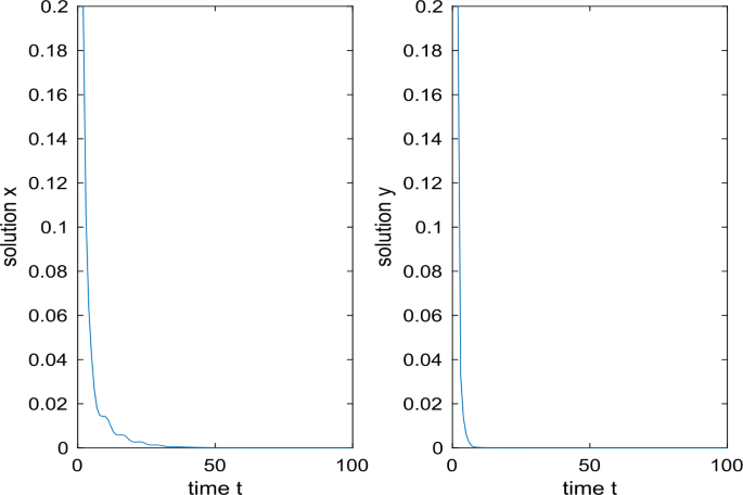
Dynamic behavior of \(x(t)\), \(y(t)\) of solution \((x(t), y(t))\) for (4.2), respectively
- \((ii)\):
-
discontinuous harvesting policy, in this case, the harvesting policies are described by the following discontinuous function:
$$ h_{1}(x, y)=h_{2}(x, y)= \textstyle\begin{cases} 0,& x+y \leq 0.5, \\ 0.5,& 0.5< x+y \leq 2, \\ 1,& x+y>2.\end{cases} $$Take the initial value as \(x(\theta ) \equiv 0.2, y(\theta )=0.2\). Figure 3 shows the dynamic behaviors of the solution \((x(t), y(t))\), which is a positive π-periodic solution of (4.2).
Figure 3 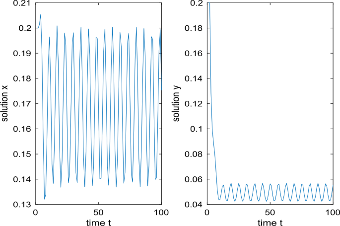
Dynamic behavior of \(x(t)\), \(y(t)\) of solution \((x(t), y(t))\) for (4.2), respectively


Note that in the case of continuous harvesting policies, excessive exploitation makes the natural resources barren, but if discontinuous harvesting policies are considered, this is conducive to the protection of natural resources and the ecological balance.
References
Aubin, J., Cellina, A.: Differential Inclusions, Set-Valued Functions and Viability Theory. Springer, Berlin (1984)
Beddington, J.R.: Mutual interference between parasites or predators and its effect on searching efficiency. J. Anim. Ecol. 44, 331–340 (1975)
Cai, Z., Huang, L.: Periodic dynamics of delayed Lotka–Volterra competition systems with discontinuous harvesting policies via differential inclusions. Chaos Solitons Fractals 54, 39–56 (2013)
Collie, J.S., Spencer, P.D.: Management strategies for fish populations subject to long-term environmental variability and depensatory predation. Tech. Rep. 93, 629–650 (1993)
Costa, M.I.S., Kaszkurewicz, E., Bhaya, A., Hsu, L.: Achieving global convergence to an equilibrium population in predator-prey systems by the use of a discontinuous harvesting policy. Ecol. Model. 128, 89–99 (2000)
DeAngelis, D.L., Goldstein, R.A., O’Neill, R.V.: A model for tropic interaction. Ecology 56, 881–892 (1975)
Fan, M., Kuang, Y.: Dynamics of a nonautonomous predator-prey system with the Beddington–DeAngelis functional response. J. Math. Anal. Appl. 295, 15–39 (2004)
Filippov, A.: Differential Equations with Discontinuous Right-Hand Side. Kluwer Academic, Boston (1988)
Guo, H., Chen, X.: Existence and global attractivity of positive periodic solution for a Volterra model with mutual interference and Beddington–DeAngelis functional respons. Appl. Math. Comput. 217, 5830–5837 (2011)
Guo, K., Ma, W.B.: Existence of positive periodic solutions for a periodic predator-prey model with fear effect and general functional responses. Adv. Cont. Discr. Mod. 22, 1–23 (2023)
Guo, Z., Zou, X.: Impact of discontinuous harvesting on fishery dynamics in a stock-effort fishing model. Commun. Nonlinear Sci. Numer. Simul. 20, 594–603 (2015)
Hassel, M.: Density dependence in single-species population. J. Anim. Ecol. 44(44), 283–295 (1975)
Huang, L., Guo, Z., Wang, J.: Theory and Applications of Differential Equationswith Discontinuous Right-Hand Sides. Science Press, Beijing (2011)
Li, H., Cheng, X.: Dynamics of stage-structured predator-prey model with Beddington–DeAngelis functional response and harvesting. Mathematics 9, 2169 (2021)
Li, W., Huang, L., Ji, J.: Periodic solution and its stability of a delayed Beddington–DeAngelis type predator-prey system with discontinuous control strategy. Math. Methods Appl. Sci. 42, 4498–4515 (2019)
Li, Y., Lin, Z.: Periodic solutions of differential inclusions. Nonlinear Anal. 24, 631–641 (1995)
Luo, D., Wang, D.: On almost periodicity of delayed predator-prey model with mutual interference and discontinuous harvesting policies. Math. Methods Appl. Sci. 39, 4311–4333 (2015)
Luo, D., Wang, D.: Impact of discontinuous harvesting policies on prey-predator system with Hassell–Varley-type functional response. Int. J. Biomath. 10, 1750048 (2017)
Luo, D., Wang, Q.: Global bifurcation and pattern formation for a reaction-diffusion predator-prey model with prey-taxis and double Beddington–DeAngelis functional responses. Nonlinear Anal., Real World Appl. 67, 103638 (2022)
Meng, Q., Yang, L.: Steady state in a cross-diffusion predator-prey model with the Beddington–DeAngelis functional response. Banach J. Math. Anal. 45, 401–413 (2019)
Ortega, V., Rebelo, C.: A note on stability criteria in the periodic Lotka–Volterra predator-prey model. Appl. Math. Lett. 145, 108739 (2023)
Wang, D., Huang, L., Cai, Z.: On the periodic dynamics of a general Cohen–Grossberg BAM neural networks via differential inclusions. Banach J. Math. Anal. 118, 203–214 (2013)
Wu, S.L., Pang, L.Y., Ruan, S.G.: Propagation dynamics in periodic predator-prey systems with nonlocal dispersal. J. Math. Pures Appl. 170, 57–95 (2023)
Xia, Z., Wu, Q., Wang, D.: Stability in terms of two measures for population growth models with impulsive perturbations. Int. J. Biomath. 13(6), 2050051 (2020)
Zeng, Z., Fan, M.: Study on a non-autonomous predator-prey system with Beddington–DeAngelis functional response. Math. Comput. Model. 48, 1755–1764 (2008)
Zhang, D., Xiong, S., Zhou, W., Ding, W.: Existence of positive periodic solution of generalized Gilpin–Ayala competition systems with discontinuous harvesting policies. Acta Ecol. Sin. 35, 107–110 (2015)
Zhang, J., Wang, J.: Periodic solutions for discrete predator-prey systems with the Beddington–DeAngelis functional response. Appl. Math. Lett. 19, 1361–1366 (2006)
Zhang, L., Fu, S.: Non-constant positive steady states for a predator-prey cross-diffusion model with Beddington–DeAngelis functional response. Bound. Value Probl. 2011, 404696 (2011)
Zhang, X., Zhao, H.: Global stability of a diffusive predator-prey model with discontinuous harvesting policy. Appl. Math. Lett. 109, 106539 (2020)
Zou, X., Li, Q., Lv, J.: Stochastic bifurcations, a necessary and sufficient condition for a stochastic Beddington–DeAngelis predator-prey model. Appl. Math. Lett. 117, Article ID 107069 (2021)
Funding
This research is supported the Natural Science Foundation of Zhejiang Province (Grant No. LY19A010013).
Author information
Authors and Affiliations
Contributions
All authors collaborated in posing the problem and creating the article. The first author wrote the main manuscript text, and the second author revise it. At the end all authors reviewed the manuscript
Corresponding author
Ethics declarations
Ethics approval and consent to participate
Not applicable.
Competing interests
The authors declare no competing interests.
Additional information
Publisher’s Note
Springer Nature remains neutral with regard to jurisdictional claims in published maps and institutional affiliations.
Rights and permissions
Open Access This article is licensed under a Creative Commons Attribution 4.0 International License, which permits use, sharing, adaptation, distribution and reproduction in any medium or format, as long as you give appropriate credit to the original author(s) and the source, provide a link to the Creative Commons licence, and indicate if changes were made. The images or other third party material in this article are included in the article’s Creative Commons licence, unless indicated otherwise in a credit line to the material. If material is not included in the article’s Creative Commons licence and your intended use is not permitted by statutory regulation or exceeds the permitted use, you will need to obtain permission directly from the copyright holder. To view a copy of this licence, visit http://creativecommons.org/licenses/by/4.0/.
About this article

Cite this article
Wang, Y., Xia, Z. Periodic dynamics of predator-prey system with Beddington–DeAngelis functional response and discontinuous harvesting. Bound Value Probl 2023, 117 (2023). https://doi.org/10.1186/s13661-023-01806-2
Received:
Accepted:
Published:
DOI: https://doi.org/10.1186/s13661-023-01806-2