The eigenvalues and sign-changing solutions of a fractional boundary value problem

Abstract

In this paper, we are interested in the eigenvalues and its algebraic multiplicities of a fractional linear boundary value problem with mixed set of Neumann and Dirichlet boundary conditions. The research results are then applied to consider the sign-changing solutions of the corresponding nonlinear problem by fixed point index and Leray-Schauder degree. To date, no paper has appeared in the literature which discusses sign-changing solutions of fractional boundary value problems. This paper attempts to fill this gap in the literature.

1 Introduction

With the development of science and technology, researchers have paid much attention to the fractional differential equations, it is extensively applied in various sciences, such as physics, mechanics, chemistry, engineering, astronomy, etc. There are a lot of research papers about the fractional differential equation boundary value problems; see [1–8] and the references therein. Most of them are devoted to the existence and multiplicity of positive solutions; see [1, 2, 6–8]. For example, in [1], the author considered the existence of positive solutions for a class of nonlinear boundary value problems of Caputo fractional equations with integral boundary conditions,

$$\textstyle\begin{cases} {}^{c}D^{\alpha}_{t}y(t)+f(y(t))=0,\quad 0< t< 1,\\ y(0)=y''(0)=0,\qquad y(1)=\lambda\int_{0}^{1}y(s)\,ds. \end{cases} $$

In [7], the author considered the existence and multiplicity of positive solutions for a nonlinear boundary value problem involving Caputo’s derivative

$$\textstyle\begin{cases} {}^{c}D^{\alpha}_{t}y(t)=f(t,y(t)),\quad t\in(0,1),\\ y(0)+y'(0)=0,\qquad y(1)+y'(1)=0. \end{cases} $$

To the best of the author’s knowledge, although sign-changing solutions of integer boundary value problems with different conditions are extensively studied by computing the algebraic multiplicities of eigenvalues, see for example [9–13] and the references therein, to date, no paper has appeared in the literature which discusses sign-changing solutions of fractional boundary value problems due to the intrinsic distinction between the eigenvalues of fractional problems and the integer problems. For example, the eigenvalues of fractional differential equations have no periodicity.

Motivated by the above papers, first, we investigate the following eigenvalue problem with the mixed set of Neumann and Dirichlet boundary conditions,

$$ \textstyle\begin{cases} {}^{c}D^{\alpha}_{t}u(t)+\lambda u(t)=0, \quad t\in(0,1),\\ u'(0)=0,\qquad u(1)=0. \end{cases} $$

(1.1)

Then we establish some existence results of sign-changing solutions for the following nonlinear fractional boundary value problem with the same boundary conditions:

$$ \textstyle\begin{cases} {}^{c}D^{\alpha}_{t}u(t)+f(u(t))=0, \quad t\in(0,1),\\ u'(0)=0,\qquad u(1)=0, \end{cases} $$

(1.2)

where $1<{\alpha}<2$ is a real number and ${}^{c}D^{\alpha}_{t}$ is the Caputo fractional derivative, $f:\mathbb{R} \mapsto\mathbb{R}$.

For convenience in the presentation, throughout this paper, let

$${\beta}_{0}=\lim_{x\rightarrow0}\frac{f(x)}{x},\qquad { \beta}_{\infty}=\lim_{x\to\infty}\frac{f(x)}{x}. $$

And we always assume the following conditions are satisfied:

• (H0) $f(x)\in C(\mathbb{R},\mathbb{R})$, $f(\theta)=\theta$, $xf(x)>0$ for all $x\in\mathbb{R}\setminus{\lbrace\theta\rbrace}$.

• (H1) There exist two positive integers $n_{0}$ and $n_{1}$. And $n_{0}$, $n_{1}$ may be equal, with

  $$\lambda_{2n_{0}}< \beta_{0}< \lambda_{2n_{0}+1},\qquad \lambda_{2n_{1}}< \beta_{\infty}< \lambda_{2n_{1}+1}, $$

  where $0<\lambda_{1}<\lambda_{2}<\cdots< \lambda_{n_{\alpha}}$ are the eigenvalues of (1.1), $n_{\alpha}$ is the number of eigenvalues.

• (H2) There exists a positive constant number $C_{0}>0$ such that $|f(x)|<\Gamma(\alpha)C_{0}$ for all x with $|x|\leq C_{0}$.

We shall organize the rest of this paper as follows. In Section 2, some basic definitions and preliminaries are given. Furthermore the eigenvalues and its algebraic multiplicities of (1.1) are considered. In Section 3, the sign-changing solutions of (1.2) are considered. An example will be given to illustrate the application in Section 4.

2 Some basic definitions and preliminaries

Definition 2.1

The Caputo fractional derivative of order $\alpha>0$ for the function $y:(0,+\infty) \to\mathbb{R}$ is defined as

$${}^{c}D_{t}^{\alpha}y(t)=\frac{1}{\Gamma(m-\alpha)} \int_{0}^{t} \frac{y^{(m)}(s)}{(t-s)^{\alpha-m+1}}\,ds, $$

where $m-1<\alpha\leq m$, and $y^{(m)}(t)$ exists.

Definition 2.2

The Riemann-Liouville fractional integral of order α for the function f is defined as

$$I_{0+}^{\alpha}f(t)=\frac{1}{\Gamma(\alpha)} \int _{0}^{t}(t-s)^{\alpha-1}f(s)\,ds, \quad \alpha>0, $$

provided that the right side is point-wise defined on $(0,\infty)$.

Definition 2.3

The Mittag-Leffler function with two parameters is defined by the series expansion

$$E_{\alpha,\beta}(z)=\sum_{k=0}^{\infty} \frac{z^{k}}{\Gamma(\alpha k+\beta)},\quad \alpha>0, \beta>0, z\in\mathbb{C}, $$

which is analytic on the whole complex plane.

Now we investigate the eigenvalue problem (1.1). From the Laplace transform of the Caputo fractional derivative [3]

$$\mathcal{L}\bigl\{ {}^{c}D^{\alpha}_{t}u(t)\bigr\} =s^{\alpha}\mathcal{L}\bigl\{ u(t)\bigr\} -\sum^{m-1}_{i=0}s^{\alpha-i-1}u^{(i)}(0),\quad m-1< \alpha\leq m, $$

and $u'(0)=0$, we have

$$\mathcal{L}\bigl\{ {}^{c}D^{\alpha}_{t}u(t)+\lambda u(t) \bigr\} =s^{\alpha }\mathcal{L}\bigl\{ u(t)\bigr\} -s^{\alpha-1}u(0) +\lambda \mathcal{L}\bigl\{ u(t)\bigr\} =0. $$

Hence

$$\mathcal{L}\bigl\{ u(t)\bigr\} =u(0)\frac{s^{\alpha-1}}{s^{\alpha}+\lambda} . $$

From the inverse Laplace transform of the Mittag-Leffler function [14]

$$E_{\alpha,1}\bigl(-\lambda t^{\alpha}\bigr)=\mathcal{L}^{-1} \biggl\{ \frac{s^{\alpha -1}}{s^{\alpha}+\lambda}\biggr\} , $$

we get

$$u(t)=u(0)E_{\alpha,1}\bigl(-\lambda t^{\alpha}\bigr). $$

By $u(1)=0$, we know

$$E_{\alpha,1}(-\lambda)=0. $$

Hence λ is the eigenvalue of (1.1) if and only if λ is a solution of $E_{\alpha,1}(-x )=0$, and for all nonzero constants $C\in \mathbb{R}$, $u(t)=CE_{\alpha,1}(-\lambda t^{\alpha})$ are the eigenfunctions corresponding eigenvalue λ.

Then we consider the inverse problem of (1.1). It follows from the definition of the Caputo fractional derivative that u is an eigenfunction of (1.1) corresponding to the eigenvalue λ, if and only if u is a solution of the integral equation

$$ u(t)= \int_{0}^{1}\lambda{G(t,s)u(s)\,ds}, $$

(2.1)

where

$$ G(t,s)=\textstyle\begin{cases} \frac{(1-s)^{\alpha-1}-(t-s)^{\alpha-1}}{\Gamma (\alpha)},& 0\leq s\leq t\leq1,\\ \frac{(1-s)^{\alpha-1}}{\Gamma(\alpha)},& 0\leq t\leq s\leq1. \end{cases} $$

(2.2)

Define the operator T as follows:

$$(Tu) (t)= \int_{0}^{t}{\frac{(1-s)^{\alpha-1}-(t-s)^{\alpha-1}}{ \Gamma(\alpha)}}u(s)\,ds+ \int_{t}^{1}{\frac{(1-s)^{\alpha-1}}{ \Gamma(\alpha)}}u(s)\,ds. $$

Therefore, we know that $\lambda\neq0$ is an eigenvalue of (1.1) if and only if $\frac{1}{\lambda}$ is an eigenvalue of operator T. That is, $\frac{1}{\lambda}$ is an eigenvalue of operator T if and only if λ is a solution of $E_{\alpha,1}(-x)=0$. And $u(t)=CE_{\alpha,1}(-\lambda t^{\alpha})$ ($C\neq0$) are the eigenfunctions corresponding to the eigenvalue $\frac{1}{\lambda}$.

Let

$$\lambda_{1}< \lambda_{2}< \cdots< \lambda_{n_{\alpha}} $$

be the sequence of solutions to the equation $E_{\alpha,1}(-x)=0$. From [5], we see that $\lambda_{j}$ ($j=1,2,\ldots,n_{\alpha}$) are positive and $n_{\alpha}$ is finite. By computing, we can get

$$n_{1.1}=n_{1.2}=n_{1.3}=n_{1.4}=1,\qquad n_{1.5}=3,\qquad n_{1.6}=5 ,\qquad n_{1.7}=9,\qquad \ldots. $$

That is, when $\alpha=1.1,1.2,1.3,1.4$, the operator T has one eigenvalue, when $\alpha=1.5$, T has three eigenvalues, when $\alpha=1.6$, T has five eigenvalues, when $\alpha=1.7$, T has nine eigenvalues, and so on. Furthermore we will consider the algebraic multiplicity of $\frac {1}{\lambda}$.

Lemma 2.1

Assume $\frac{1}{\lambda}$ is the eigenvalue of T, that is, $E_{\alpha,1}(-\lambda)=0$. Furthermore $E_{\alpha ,1}^{(1)}(-\lambda)\neq0$. Then the algebraic multiplicity of eigenvalue $\frac{1}{\lambda}$ for T is equal to 1.

Proof

It is obvious that

$$\operatorname{ker}(I-\lambda T)\subseteq \operatorname{ker}(I-\lambda T)^{2}. $$

Let $u\in \operatorname{ker}(I-\lambda T)^{2}$, if $u\notin \operatorname{ker}(I-\lambda T)$, then there exists a nonzero constant C such that

$$\bigl((I-\lambda T)u\bigr) (t)=CE_{\alpha, 1}\bigl(-\lambda t^{\alpha} \bigr), \quad t\in(0,1), $$

since $CE_{\alpha, 1}(-\lambda t^{\alpha})$ ($C\neq0$) are the eigenfunctions of operator T corresponding to the eigenvalue $\frac {1}{\lambda}$. By direct computation, we have

$$ \textstyle\begin{cases} D^{\alpha}u(t) +\lambda u(t)=-C\lambda E_{\alpha,1}(-\lambda t^{\alpha}),\quad t\in (0,1),\\ u'(0)=0, \qquad u(1)=0. \end{cases} $$

(2.3)

From the Laplace transform of the Caputo fractional derivative [3],

$$\mathcal{L}\bigl\{ D^{\alpha}u(t)\bigr\} =s^{\alpha}\mathcal{L}\bigl\{ u(t)\bigr\} -\sum^{m-1}_{i=0}s^{\alpha-i-1}u^{(i)}(0),\quad m-1< \alpha\leq m, $$

the Laplace transform of the Mittag-Leffler function [14],

$$\mathcal{L}\bigl\{ t^{\mu-1}E_{\alpha,\mu}\bigl(-\lambda t^{\alpha} \bigr)\bigr\} =\frac {s^{\alpha-\mu}}{s^{\alpha}+\lambda}, $$

and $u'(0)=0$, we have

$$s^{\alpha}\mathcal{L}\bigl\{ u(t)\bigr\} -s^{\alpha-1}u(0) +\lambda \mathcal{L}\bigl\{ u(t)\bigr\} = -\frac{C\lambda s^{\alpha-1}}{s^{\alpha}+\lambda}. $$

Hence

$$\mathcal{L}\bigl\{ u(t)\bigr\} =u(0)\frac{s^{\alpha-1}}{s^{\alpha}+\lambda} -\frac{C\lambda s^{\alpha-1}}{(s^{\alpha}+\lambda )^{2}}. $$

From the inverse Laplace transform of the Mittag-Leffler function [14],

$$t^{m\rho+\beta-1}E_{\rho,\beta}^{(m)}\bigl(-\lambda t^{\rho} \bigr)=\mathcal{L}^{-1} \biggl\{ \frac{m!s^{\rho-\beta}}{(s^{\rho} +\lambda)^{m+1}}\biggr\} \quad\mbox{with } E_{\rho,\beta}^{(m)}(z)=\frac {d^{m}}{dz^{m}} E_{\rho,\beta}(z), $$

we can obtain

$$ u(t)=u(0)E_{\alpha,1}\bigl(-\lambda t^{\alpha}\bigr) -C\lambda t^{\alpha}E_{\alpha, 1}^{(1)}\bigl(-\lambda t^{\alpha} \bigr). $$

(2.4)

Let $u(1)=0$, then we get

$$E_{\alpha, 1}^{(1)}(-\lambda)=0, $$

which is a contradiction. Hence $u\in \operatorname{ker}(I-\lambda T)$, that is,

$$\operatorname{ker}(I-\lambda T)^{2}\subseteq \operatorname{ker}(I-\lambda T). $$

Therefore

$$\operatorname{ker}(I-\lambda T)^{2}= \operatorname{ker}(I-\lambda T). $$

By

$$\operatorname{dim} \operatorname{ker} \biggl(\frac{1}{\lambda}I-T\biggr)=\operatorname{dim} \operatorname{ker}(I-\lambda T)=\operatorname{dim} \operatorname{ker}(I- \lambda T)^{2}=\operatorname{dim} \operatorname{ker}\biggl(\frac{1}{\lambda}I-T\biggr)^{2}, $$

we see that the algebraic multiplicity of the eigenvalue $\frac {1}{\lambda}$ is equal to 1. This completes the proof. □

Lemma 2.2

Assume $\frac{1}{\lambda}$ is the eigenvalue of T, that is, $E_{\alpha,1}(-\lambda)=0$. Furthermore $E_{\alpha ,1}^{(1)}(-\lambda)=E_{\alpha,2}^{(1)}(-\lambda)=0$, $E_{\alpha ,1}^{(2)}(-\lambda)\neq0$. Then the algebraic multiplicity of the positive eigenvalue $\frac{1}{\lambda}$ for T is equal to 2.

Proof

By Lemma 2.1, we know that, if $E_{\alpha,1}^{(1)}(-\lambda)=0$, then

$$\operatorname{ker}(I-\lambda T)^{2}\nsubseteq \operatorname{ker}(I-\lambda T). $$

It is obvious that

$$\operatorname{ker}(I-\lambda T)\subseteq \operatorname{ker}(I-\lambda T)^{2}\subseteq \operatorname{ker}(I-\lambda T)^{3}. $$

Then we need to show

$$\operatorname{ker}(I-\lambda T)^{3}\subseteq \operatorname{ker}(I-\lambda T)^{2}. $$

Let $u\in \operatorname{ker}(I-\lambda T)^{3}$, if $u\notin \operatorname{ker}(I-\lambda T)^{2}$, then there exists a nonzero constant C such that

$$\bigl((I-\lambda T)^{2}u\bigr) (t)=CE_{\alpha, 1}\bigl(-\lambda t^{\alpha}\bigr),\quad t\in(0,1). $$

By direct computation, we have

$$ \textstyle\begin{cases} D^{\alpha} (D^{\alpha}u(t)+\lambda u(t)) +\lambda(D^{\alpha}u(t)+\lambda u(t))=C\lambda^{2} E_{\alpha ,1}(-\lambda t^{\alpha}),\quad t\in(0,1),\\ u'(0)=0, \qquad u(1)=0. \end{cases} $$

(2.5)

Let $v=D^{\alpha}u(t)+\lambda u(t)$, by Lemma 2.1, we see that

$$ D^{\alpha}u(t)+\lambda u(t)=v(t)=v(0)E_{\alpha,1}\bigl(-\lambda t^{\alpha }\bigr)+v'(0)t E_{\alpha,2}\bigl(-\lambda t^{\alpha}\bigr) +C\lambda^{2} t^{\alpha}E_{\alpha, 1}^{(1)} \bigl(-\lambda t^{\alpha}\bigr). $$

(2.6)

From the Laplace transform of the Caputo fractional derivative, the Laplace transform of the Mittag-Leffler function [3, 14] and $u'(0)=0$, we have

$$s^{\alpha}\mathcal{L}\bigl\{ u(t)\bigr\} -s^{\alpha-1}u(0) + \lambda_{k}\mathcal{L}\bigl\{ u(t)\bigr\} =v(0)\frac{s^{\alpha-1}}{s^{\alpha}+\lambda} +v'(0)\frac{s^{\alpha-2}}{s^{\alpha}+\lambda} +\frac{C\lambda^{2} s^{\alpha-1}}{(s^{\alpha}+\lambda)^{2}}. $$

Hence

$$\mathcal{L}\bigl\{ u(t)\bigr\} =u(0)\frac{s^{\alpha-1}}{s^{\alpha}+\lambda} +v(0)\frac{s^{\alpha-1}}{(s^{\alpha}+\lambda)^{2}} +v'(0)\frac{s^{\alpha-2}}{(s^{\alpha}+\lambda)^{2}} +\frac{C\lambda^{2} s^{\alpha-1}}{(s^{\alpha}+\lambda)^{3}}. $$

From the inverse Laplace transform of the Mittag-Leffler function [14], we can obtain

$$\begin{aligned} u(t) =&u(0)E_{\alpha,1}\bigl(-\lambda t^{\alpha}\bigr) +v(0)t^{\alpha}E_{\alpha,1}^{(1)}\bigl(-\lambda t^{\alpha} \bigr) +v'(0)t^{\alpha+1}E_{\alpha,2}^{(1)}\bigl(- \lambda t^{\alpha}\bigr) \\ &{} +C\lambda t^{2\alpha}E_{\alpha, 1}^{(2)} \bigl(-\lambda t^{\alpha}\bigr). \end{aligned}$$

(2.7)

Let $u(1)=0$, then we get

$$E_{\alpha, 1}^{(2)}(-\lambda)=0, $$

which is a contradiction. Hence

$$\operatorname{ker}(I-\lambda T)^{3}\subseteq \operatorname{ker}(I-\lambda T)^{2}. $$

Therefore

$$\operatorname{ker}(I-\lambda T)^{3}= \operatorname{ker}(I-\lambda T)^{2}. $$

That is, the algebraic multiplicity of the eigenvalue $\frac {1}{\lambda}$ is equal to 2. This completes the proof. □

Similarly to Lemma 2.1, Lemma 2.2, we can study the algebraic multiplicity of eigenvalue $\frac{1}{\lambda}$ for operator T by Laplace transforms. Then we will consider the sign-changing solutions of (1.2) by the algebraic multiplicity of the eigenvalue $\frac{1}{\lambda}$ for the operator T.

3 The existence of sign-changing solutions

Consider the Banach space

$$E=\bigl\{ u\in C^{1}[0,1]:u'{(0)}=0,u(1)=0\bigr\} $$

with the norm $\|u\|=\max\{\|u\|_{\infty},\|u'\|_{\infty}\}$, where $\|u\|_{\infty}=\max_{{0}\leq{t}\leq{1}}{| u(t)|}$. Let

$$P=\bigl\{ u\in E:u(t)\ge0, \forall t\in[0,1]\bigr\} $$

be a cone of E. Define operators F and B as follows:

$$(Fu) (t)=f\bigl(u(t)\bigr),\quad t\in(0,1), u\in E $$

and

$$B=T\circ F. $$

Then u is a solution of (1.2) if and only if u is a solution of the operator equation

$$u=Bu. $$

By (H0), we can see that B, T are completely continuous.

Lemma 3.1

Assume that (H0) hold, then the operator B is Fréchet differentiable at θ and ∞, and $B'(\theta )=\beta_{0}T$, $B'(\infty)=\beta_{\infty}T$.

Proof

From ${\beta}_{0}=\lim_{x\rightarrow0}\frac{f(x)}{x}$, we have $\forall \varepsilon> 0$, $\exists {\delta} > 0$, $\forall 0<|x|<\delta$, and we see that

$$\biggl|{\frac{f(x)}{x}}-\beta_{0} \biggr|< \varepsilon, $$

that is, $|f(x)-\beta_{0}x|<\varepsilon|x|$. Assume that $\|u\|_{\infty}\leq\delta$, then by (H0), we have

$$\begin{aligned} \bigl|(Bu-B\theta-\beta_{0}Tu) (t)\bigr| =&\bigl|\bigl(T(Fu-\beta_{0})u \bigr) (t)\bigr|< \varepsilon\| u \|_{\infty} \int_{0}^{1}G(t,s) \,ds \\ < &\varepsilon\|u \| \int_{0}^{1}\frac{(1-s)^{\alpha-1}}{\Gamma (\alpha)}\,ds = \frac{\|u\|}{ \Gamma(\alpha+1)}\varepsilon. \end{aligned}$$

That implies

$$\|{Bu-B\theta-\beta_{0}Tu}\|_{\infty} < \frac{\|u\|}{ \Gamma(\alpha +1)} \varepsilon,\quad \forall u\in E. $$

Similarly, we can show that

$$\bigl\| (Bu-B\theta-\beta_{0}Tu)'(t)\bigr\| _{\infty} < \frac{\|u\|}{\Gamma(\alpha)}\varepsilon. $$

Hence

$$\bigl\| {Bu-B\theta-\beta_{0}Tu}\bigr\| < \max\biggl\{ \frac{1}{ \Gamma(\alpha+1)}, \frac{1}{\Gamma(\alpha)}\biggr\} \|u\|\varepsilon=\frac{\| u \|}{\Gamma (\alpha)}\varepsilon. $$

Consequently

$$ \lim_{\|u\|\rightarrow0} \frac{\|{Bu-B\theta-\beta _{0}Tu}\|}{\|u\|}=0. $$

(3.1)

This means that B is Fréchet differentiable at θ, and $B'(\theta)=\beta_{0}T$.

From ${\beta}_{\infty}=\lim_{x\rightarrow\infty}\frac{f(x)}{x}$, we have $\forall \varepsilon> 0$; let $N>0$, when $|x|>N$, we have

$$\biggl|{\frac{f(x)}{x}}-\beta_{\infty} \biggr|< \varepsilon, $$

that is, $|f(x)-\beta_{\infty}x|<\varepsilon|x|$. Make $M=\max_{|x|\leq N}|{f(x)-\beta_{\infty}x}|$, then we have

$$\bigl|f(x)-\beta_{\infty}x\bigr|< \varepsilon|x|+M. $$

Hence, assume that $\|u\|_{\infty}>N$, by (H0), we see that

$$\begin{aligned} \bigl|(Bu-\beta_{\infty}Tu) (t)\bigr| =&\bigl| T(Fu-\beta_{\infty}u) (t)\bigr|< \bigl(\varepsilon \|u\|_{\infty} + M\bigr) \int_{0}^{t}G(t,s)\,ds \\ < &\bigl(\varepsilon\|u\| + M\bigr) \int_{0}^{1}\frac{(1-s)^{\alpha-1}}{\Gamma (\alpha)}\,ds = \frac{1}{\Gamma(\alpha+1)}\bigl(\varepsilon\|u\|+M\bigr). \end{aligned}$$

That implies that

$$\| Bu-\beta_{\infty} Tu\|_{\infty} < \frac{1}{\Gamma (\alpha+1)}\bigl( \varepsilon\|u\| + M\bigr),\quad u\in E. $$

Similarly, we can show that

$$\bigl\| (Bu-\beta_{\infty} Tu)'\bigr\| _{\infty} < \frac{1}{\Gamma (\alpha)}\bigl(\varepsilon\| u\| + M\bigr),\quad u\in E. $$

Hence

$$\| Bu-\beta_{\infty} Tu\|< \frac{1}{\Gamma(\alpha)}\bigl(\varepsilon\| u\| + M\bigr). $$

Consequently

$$ \lim_{\| u \| \rightarrow\infty} \frac{\| {Bu-\beta_{\infty}Tu}\| }{\| u \|}=0. $$

(3.2)

Therefore B is Fréchet differentiable at ∞, and $B'(\infty)=\beta_{\infty}T$. □

Lemma 3.2

Assume that (H0) hold, $u\in P\setminus{\lbrace\theta\rbrace }$ is a solution of (1.2), then $u\in\mathring{P}$.

Proof

If $u\in P\setminus\{ \theta\}$ is a solution of (1.2), then

$$\begin{aligned}& u(t)= \int_{0}^{1}G(t,s)f\bigl(u(s)\bigr)\,ds \\& \hphantom{u(t)}= \int_{0}^{t}\frac{(1-s)^{\alpha-1}-(t-s)^{\alpha-1}}{\Gamma (\alpha)}f\bigl(u(s)\bigr)\,ds + \int_{t}^{1}\frac{(1-s)^{\alpha-1}}{\Gamma(\alpha)}f\bigl(u(s)\bigr)\,ds, \\& u'(t)=-\frac{1}{\Gamma(\alpha)} \int_{0}^{t} (\alpha -1) (t-s)^{\alpha-2}f \bigl(u(s)\bigr)\,ds. \end{aligned}$$

It is obvious that

$$u'(0)=0,\qquad u(1)=0, \qquad u(0)>0,\qquad u'(1)< 0,\qquad u'(t)< 0. $$

From $u'(1)<0$ we learn that there exist $\varepsilon>0$, $\tau_{1}>0$, such that

$$ u'(t)< -\tau_{1}, \quad \forall t\in[1-\varepsilon,1]. $$

(3.3)

From $u(1)=0$, $u'(t)<0$, $\forall t\in(0,1]$ we learn that there exists $\tau_{2}>0$, such that

$$ u(t)>\tau_{2}, \quad \forall t\in[0,1-\varepsilon]. $$

(3.4)

Let $\tau= \min(\tau_{1},\tau_{2})$, then if $\| x-u \| < \tau$ for any $x\in E$, we can get $x(t)\geq0$, $t\in[0,1]$ by (3.4), (3.5), that is, $x\in P$. Consequently $B(u,\tau)\subset P$ and $u\in\mathring{P}$. □

Lemma 3.3

([15])

Let P be a solid cone of real Banach space E, Ω be a relatively bounded open set of P, $A:P\mapsto P$ be a completely continuous operator. If all fixed points of A are an interior point of P, there exists an open subset O of E such that $O\subset\Omega$ and $\operatorname{deg}(I-A,O,\theta)=i(A,\Omega, P)$.

Theorem 3.4

Suppose that (H0)-(H2) hold, $0<\lambda_{1}<\lambda _{2}<\cdots< \lambda_{n_{\alpha}}$ are the eigenvalues of (1.1). Furthermore $E^{(1)}_{\alpha,1}(-\lambda_{j})\neq0$, where $j=1,2,\ldots,\max\{2n_{0},2n_{1}\}$. Then the boundary value problem (1.2) has at least two sign-changing solutions, two positive solutions and two negative solutions.

Proof

It follows from the definition of B that u is a solution of (1.2) if and only if u is the fixed point of the operator B. Then by (H2), we have, for any $u\in E$ with $\|u\| = C_{0}$,

$$\begin{aligned}& \bigl|(Bu)(t)\bigr|= \biggl|-\int_{0}^{t}\frac{(t-s)^{\alpha-1}}{\Gamma (\alpha)}f\bigl(u(s)\bigr)\,ds +\int_{0}^{1}\frac{(1-s)^{\alpha-1}}{\Gamma(\alpha)}f\bigl(u(s)\bigr)\,ds \biggr|\\& \hphantom{ \bigl|(Bu)(t)\bigr|}< \Gamma(\alpha)C_{0}\int_{0}^{1}\frac{(1-s)^{\alpha-1}}{\Gamma (\alpha)} \,ds\\& \hphantom{ \bigl|(Bu)(t)\bigr|}< C_{0},\\& \bigl|(Bu)'(t)\bigr|= \biggl|-\frac{1}{\Gamma(\alpha)}\int_{0}^{t}(\alpha -1)(t-s)^{\alpha-2}f\bigl(u(s)\bigr)\,ds \biggr|\\& \hphantom{\bigl|(Bu)'(t)\bigr|}< \Gamma(\alpha)C_{0}\frac{\alpha-1}{\Gamma(\alpha)}\int _{0}^{1}(1-s)^{\alpha-2} \,ds\\& \hphantom{\bigl|(Bu)'(t)\bigr|} =C_{0}. \end{aligned}$$

Therefore $\| Bu \| < C_{0}$. By (H0) and $G(t,s)\geq0$, we have $B(P)\subset P$. Hence

$$ i\bigl(B,P \cap B(\theta,C_{0}),P\bigr)=1. $$

(3.5)

By Lemma 3.3, we see that

$$ \operatorname{deg}\bigl(I-B, B(\theta,C_{0}),\theta\bigr)=1. $$

(3.6)

By Lemma 3.1, we can learn that $B'(\theta)=\beta_{0}T$. Hence $\frac{\beta_{0}}{\lambda_{j}}$ ($j=1,2,\ldots,n_{\alpha}$) are the eigenvalues of the operator $B'(\theta)$. By (H1), we know that $\frac{\beta_{0}}{\lambda_{1}}>1$. Hence 1 is not an eigenvalue of $B'(\theta)$. Furthermore, $u(t)=CE_{\alpha,1}(-\lambda_{1}t^{\alpha})$ ($C\neq0$) is an eigenfunction of $B'(\theta)$ corresponding to the eigenvalue $\lambda_{1}$. And $E_{\alpha, 1}(-\lambda_{1}t^{\alpha})\neq0$ for any $t\in(0,1)$, since $\lambda_{1}$ is the smallest positive solution of $E_{\alpha, 1}(-x)=0$. Hence we can choose the suitable C to ensure $u(t)\geq0$. Therefore, by Theorem 21.2, in [16], we know that there exist a small enough $r_{1}$ and a large enough $R_{1}$ such that

$$\begin{aligned}& \operatorname{deg}\bigl(I-B,U(\theta,r_{1}),\theta\bigr)=(-1)^{k_{0}}, \end{aligned}$$

(3.7)

$$\begin{aligned}& \operatorname{deg}\bigl(I-B,U(\theta,R_{1}),\theta\bigr)=(-1)^{k_{1}}, \end{aligned}$$

(3.8)

where $k_{0}$ is the sum of the algebraic multiplicities of the real eigenvalues of $B'(\theta)$ which are larger than 1, $k_{1}$ is the sum of the algebraic multiplicities of the real eigenvalues of $B'(\infty)$ which are larger than 1.

By Lemma 2.3.7 in [17], we see that there exist two constants $r_{0}$, $R_{0}$ ($0< r_{0}< C_{0}< R_{0}$) such that for any $r_{1}$, $R_{1}$ ($0< r_{1}< r_{0}< C_{0}< R_{0}< R_{1}$),

$$\begin{aligned}& i\bigl(B,P \cap U(\theta,r_{1}),P\bigr)=0, \end{aligned}$$

(3.9)

$$\begin{aligned}& i\bigl(B,P \cap U(\theta,R_{1}),P\bigr)=0. \end{aligned}$$

(3.10)

Hence, by (3.5), (3.9), (3.10), we see that

$$\begin{aligned}& i\bigl(B,P \cap\bigl(U(\theta,R_{1})\setminus\overline{U( \theta,C_{0})}\bigr),P\bigr)=0-1=-1, \end{aligned}$$

(3.11)

$$\begin{aligned}& i\bigl(B,P \cap\bigl(U(\theta,C_{0})\setminus\overline{U( \theta,r_{1})}\bigr),P\bigr)=1-0=1. \end{aligned}$$

(3.12)

Therefore the operator B has at least two fixed points

$$u_{1} \in P \cap\bigl(U(\theta,R_{1})\setminus\overline{U( \theta ,C_{0})}\bigr),\qquad u_{2}\in P \cap\bigl(U( \theta,C_{0})\setminus\overline {U(\theta,r_{1})}\bigr). $$

That is, $u_{1}$ and $u_{2}$ are positive solutions of the boundary value problem (1.2) and $r_{1}<\|u_{1}\|\leq C_{0}$ and $C_{0}<\|u_{2}\| \leq R_{1}$.

By (H0), we have $uf(u)>0$ for all $u\in\mathbb{R}\setminus{\lbrace \theta\rbrace}$. Similarly, we see that boundary value problem (1.2) has two negative solutions $u_{3},u_{4}\in-P$ with

$$-u_{3} \in P \cap\bigl(U(\theta,R_{1})\setminus\overline{U( \theta ,C_{0})}\bigr),\qquad -u_{4}\in P \cap\bigl(U( \theta,C_{0})\setminus\overline {U(\theta,r_{1})}\bigr) $$

and $r_{1}<\|u_{3}\|\leq C_{0}$, $C_{0}<\|u_{4}\|\leq R_{1}$.

By (3.11), (3.12), and Lemma 3.3. there exist two open subsets $O_{1}$, $O_{2}$ of E

$$O_{1} \subset P \cap\bigl(U(\theta,C_{0})\setminus \overline{U(\theta ,r_{1})}\bigr),\qquad O_{2}\subset P \cap \bigl(U(\theta,R_{1})\setminus\overline {U(\theta,C_{0})} \bigr), $$

such that

$$\begin{aligned}& \operatorname{deg}(I-B,O_{1},\theta)=1, \end{aligned}$$

(3.13)

$$\begin{aligned}& \operatorname{deg}(I-B,O_{2},\theta)=-1. \end{aligned}$$

(3.14)

Similarly, there exist two open subsets $O_{3}$, $O_{4}$ of E

$$O_{3} \subset-P \cap\bigl(U(\theta,C_{0})\setminus \overline{U(\theta ,r_{1})}\bigr), \qquad O_{4} \subset-P \cap \bigl(U(\theta,R_{1})\setminus\overline {U(\theta,C_{0})} \bigr), $$

such that

$$\begin{aligned}& \operatorname{deg}(I-B,O_{3},\theta)=1, \end{aligned}$$

(3.15)

$$\begin{aligned}& \operatorname{deg}(I-B,O_{4},\theta)=-1, \end{aligned}$$

(3.16)

by (H0).

By (H1) and Lemma 3.1, the number of eigenvalues of the operator $B'(\theta)=\beta_{0}K$ which are larger than 1 is $2n_{0}$. From

$$E^{(1)}_{\alpha,1}(-\lambda_{j})\neq0, $$

$j=1,2,\ldots,\max\{2n_{0},2n_{1}\}$ and Lemma 2.1 we see that the algebraic multiplicity of positive eigenvalue $\frac{\beta _{0}}{\lambda_{n}}$ have algebraic multiplicity one. Hence $k_{0}=2n_{0}$, and

$$ \operatorname{deg}\bigl(I-B,U(\theta,r_{1}),\theta\bigr)=(-1)^{k_{0}}=(-1)^{2n_{0}}=1. $$

(3.17)

Similarly we can see that

$$ \operatorname{deg}\bigl(I-B,U(\theta,R_{1}),\theta\bigr)=(-1)^{k_{1}}=(-1)^{2n_{1}}=1. $$

(3.18)

From (3.6), (3.13), (3.15), and (3.17) we see that

$$ \operatorname{deg}\bigl(I-B,U(\theta,C_{0})\setminus\bigl(\overline{O_{1}} \cup\overline {O_{3}} \cup\overline{U(\theta,r_{1})}\bigr), \theta\bigr)=1-1-1-1=-2. $$

(3.19)

By (3.19), we know B has at least one fixed point $u_{5}\in U(\theta ,C_{0})\setminus(\overline{O_{1}} \cup\overline{O_{3}} \cup \overline{U(\theta,r_{1})})$.

That is, boundary value problem (1.2) has a sign-changing solution $u_{5}$. Similarly, we get another different solution $u_{6}\in U(\theta,C_{0})\setminus(\overline{O_{2}} \cup\overline{O_{4}} \cup\overline{U(\theta,C_{0})})$ by (3.6), (3.14), (3.16), and (3.18). This completes the proof. □

According to the method used in the proof of Theorem 3.4, we can give the following corollaries.

Corollary 3.5

Let (H0)-(H2) hold, $0<\lambda_{1}<\lambda _{2}<\cdots<\lambda_{n_{\alpha}}$ are the eigenvalues of (1.1), there exists a positive integer $n_{0}$ such that $\lambda_{2n_{0}} <\beta_{0} < \lambda_{2n_{0}+1}$ or $\lambda_{2n_{0}} <\beta_{\infty} < \lambda _{2n_{0}+1}$ and $E^{(1)}_{\alpha,1}(-\lambda_{j})\neq0$, where $j=1,2,\ldots,2n_{0}$. Then the boundary value problem (1.2) have at least one sign-changing solution, one positive solution and one negative solution.

Corollary 3.6

Let (H0)-(H2) hold, $\lambda_{1}$ is the eigenvalue of (1.1), $E^{(1)}_{\alpha ,1}(-\lambda_{1})\neq0$.

• (1) If $\beta_{\infty}<\lambda_{1} <\beta_{0}$ or $\beta_{0}<\lambda_{1} <\beta_{\infty}$, then the boundary value problem (1.2) has at least one positive solution and one negative solution.

• (2) If $\beta_{0}>\lambda_{1}$, $\beta_{\infty}>\lambda_{1}$, then the boundary value problem (1.2) has at least two positive solutions and two negative solutions.

4 Example

Consider the following fractional differential equation:

$$ \textstyle\begin{cases} {}^{c}D^{1.5}_{x}u(t)+f(u(t))=0, \quad t\in(0,1),\\ u'(0)=0,\qquad u(1)=0, \end{cases} $$

(4.1)

where

$$ f(u)=\textstyle\begin{cases} -\frac{1}{2}, & u \leq-\frac{1}{28},\\ 14u,& -\frac{1}{28}< u < \frac{1}{28},\\ \frac{1}{2}, & \frac{1}{28}\leq u. \end{cases} $$

(4.2)

We can find that

• (1) $\beta_{0}=\lim_{u\rightarrow0}\frac{f(u)}{u}=14$;

• (2) $f(u):\mathbb{R} \mapsto\mathbb{R}$, $f(\theta)=\theta$, $uf(u)>0$ for all $t\in(0,1)$, $u\in\mathbb{R}\setminus{\lbrace\theta\rbrace }$;

• (3) from [4, 5], we see that $E_{1.5 ,1}(-x)=0$ has three zero points, $x_{1}= 2.11$, $x_{2}= 13.765$, $x_{3}=24.243$, and $E^{(1)}_{\alpha,1}(-x_{1})\neq0$, $E^{(1)}_{\alpha,1}(-x_{2})\neq0$;

• (4) $\lambda_{2}<\beta_{0}<\lambda_{3}$;

• (5) let $C_{0}=1$, when $-\frac{1}{28}< u<\frac{1}{28}$, we have

  $$\bigl| f(u) \bigr|=| 14 u |\leq\frac{1}{2} < \Gamma(1.5) $$

  when $u \leq-\frac{1}{28}$ or $\frac{1}{28}\leq u$, we have

  $$\bigl| f(u) \bigr| = \frac{1 }{2}< \Gamma(1.5). $$

  By Corollary 3.5, we see that problem (4.1) has at least one sign-changing solution $u_{1}$, one positive solution $u_{2}$, one negative solution $u_{3}$. By $f(-u)=-f(u)$, we see that $u_{4}=-u_{1}$ is another sign-changing solution of (4.1). The numerical results of $u_{1}$, $u_{2}$, $u_{3}$ and $u_{4}$ are shown in Table 1, the graphs of $u_{1}$, $u_{2}$, $u_{3}$ and $u_{4}$ are shown in Figure 1.

  Figure 1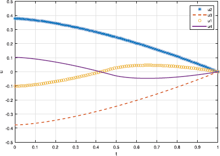

  

  Sign-changing solutions $\pmb{u_{1}}$ , $\pmb{u_{4}}$ , positive solution $\pmb{u_{2}}$ , negative solution $\pmb{u_{3}}$ .

  Table 1 Sign-changing solutions $\pmb{u_{1}}$ , $\pmb{u_{4}}$ , positive solution $\pmb{u_{2}}$ , negative solution $\pmb{u_{3}}$

5 Conclusion

In the paper, the existence of sign-changing solutions for a fractional boundary value problem is considered by the eigenvalues. Some new results as regards the eigenvalues and their algebraic multiplicities are established. Finally, an example is presented to illustrate the application.

References

Cabada, A, Wang, GT: Positive solutions of nonlinear fractional differential equations with integral boundary value conditions. J. Math. Anal. Appl. 389, 403-411 (2012)
Jiang, DQ, Yuan, CJ: The positive properties of the Green function for Dirichlet-type boundary value problems of nonlinear fractional differential equations and its application. Nonlinear Anal. 72, 710-719 (2010)
Saei, FD, Abbasi, S, Mirzayi, Z: Inverse Laplace transform method for multiple solutions of the fractional Sturm-Liouville problems. Comput. Methods Differ. Equ. 2, 56-61 (2014)
Duan, JS, Wang, Z, Liu, YL, Qiu, X: Eigenvalue problems for fractional ordinary differential equations. Chaos Solitons Fractals 46, 46-53 (2013)
Sabatier, J, Agarwal, OP, Tenreiro Machado, JA: Advances in Fractional Calculus, Theoretical Developments and Applications in Physics and Engineering. Springer, Berlin (2007)
Liang, SH, Zhang, JH: Positive solutions for boundary value problems of nonlinear fractional differential equation. Nonlinear Anal. 71, 5545-5550 (2009)
Zhang, SQ: Positive solutions for boundary value problems of nonlinear fractional differential equations. Electron. J. Differ. Equ. 2006, 36 (2006)
Bai, ZB, Lü, HS: Positive solutions for boundary value problems of nonlinear fractional differential equation. J. Math. Anal. Appl. 311, 495-505 (2005)
Li, FY, Zhang, YB, Li, YH: Sign-changing solutions on a kind of fourth-order Neumann boundary value problem. J. Math. Anal. Appl. 344, 417-428 (2008)
Zhang, KM, Xie, XJ: Existence of sign-changing solutions for some asymptotically linear three-point boundary value problems. Nonlinear Anal. 70, 2796-2805 (2009)
Lu, SS: Signed and sign-changing solutions for a Kirchhoff-type equation in bounded domains. J. Math. Anal. Appl. 432, 965-982 (2015)
Xu, X: Multiple sign-changing solutions for some m-point boundary-value problems. Electron. J. Differ. Equ. 2004, 89 (2004)
Li, YH, Li, FY: Sign-changing solutions to second-order integral boundary value problems. Nonlinear Anal. 69, 1179-1187 (2008)
Gorenflo, R, Kilbas, AA, Mainardi, F, Rogosin, SV: Mittag-Leffler Functions, Related Topics and Application. Springer, Berlin (2014)
Wei, ZL, Pang, CC: Multiple sign-changing solutions for fourth order m-point boundary value problems. Nonlinear Anal. 66, 839-855 (2007)
Krasnosel’skii, MA, Zabreiko, PP: Geometrical Methods of Nonlinear Analysis. Springer, Berlin (1984)
Guo, DJ, Lakshmikantham, V: Nonlinear Problems in Abstract Cones. Academic Press, New York (1988)
Acknowledgements
The authors thank for the editors and referees for valuable comments. This work was supported by the Fundamental Research Funds for the Central Universities.
Author information
Authors and Affiliations
Corresponding author
Additional information
Competing interests
The authors declare that they have no competing interests.
Authors’ contributions
XZ raised these interesting problems. All authors contributed to the proofs of the main results and approved the final version of the manuscript.
Rights and permissions
Open Access This article is distributed under the terms of the Creative Commons Attribution 4.0 International License (http://creativecommons.org/licenses/by/4.0/), which permits unrestricted use, distribution, and reproduction in any medium, provided you give appropriate credit to the original author(s) and the source, provide a link to the Creative Commons license, and indicate if changes were made.
About this article
Cite this article
Zhao, X., An, F. The eigenvalues and sign-changing solutions of a fractional boundary value problem. Adv Differ Equ 2016, 109 (2016). https://doi.org/10.1186/s13662-016-0838-y
Received:
Accepted:
Published:
DOI: https://doi.org/10.1186/s13662-016-0838-y