
Abstract
Soundscapes have been likened to acoustic landscapes, encompassing all the acoustic features of an area. The sounds that make up a soundscape can be grouped according to their source into biophony (sounds from animals), geophony (sounds from atmospheric and geophysical events), and anthropophony (sounds from human activities). Natural soundscapes have changed over time because of human activities that generate sound, alter land-use patterns, remove animals from natural settings, and result in climate change. These human activities have direct and indirect effects on animal distribution patterns and (acoustic) behavior. Consequently, current soundscapes may be very different from those a few hundred years ago. This is of concern as natural soundscapes have ecological value. Losing natural soundscapes may, therefore, result in a loss of biodiversity and ecosystem functioning. The study of soundscapes can identify ecosystems undergoing change and potentially document causes (such as noise from human activities). Methods for studying soundscapes range from listening and creating visual (spectrographic) displays to the computation of acoustic indices and advanced statistical modeling. Passive acoustic recording has become an ecological tool for research, monitoring, and ultimately conservation management. This chapter introduces terrestrial and aquatic soundscapes, soundscape analysis tools, and soundscape management.
Jeanette A. Thomas (deceased) contributed to this chapter while at the Department of Biological Sciences, Western Illinois University-Quad Cities, Moline, IL, USA
You have full access to this open access chapter, Download chapter PDF
7.1 Introduction
Whether listening in a forest or on an open plain, by the side of a river or in the ocean, at the outskirts of suburbia or right downtown, the Earth abounds with sounds. The use of the term “soundscape” in the literature has increased rapidly since 2000 (Fig. 7.1) and can be traced back to Southworth’s (1969) article on the sonic environment of Boston, MA, USA. The Canadian music composer and researcher Schafer later defined soundscapes as “the auditory properties of landscapes” (Schafer 1977). Schafer was a pioneer in highlighting the need for soundscape research and management. In his book, The New Soundscape, Schafer and his students documented rapid changes in soundscapes over the course of human civilization (Schafer 1969). Common settings of primitive cultures surrounded by an abundance of natural sounds (i.e., wind, water, animals, etc.) rapidly changed after the Industrial Revolution to cities dominated by sounds from machinery. Schafer further noticed that most people had ceased to listen to the sounds of the environment and actively tried to ignore unpleasant sound (i.e., noise). With the goals of studying and archiving soundscapes, creating public awareness of noise pollution, and creating healthy soundscapes through acoustic design, Schafer founded the World Soundscape Project (WSP 1972–1979; Torigoe 1982). Soundscape studies by the WSP were human-centered, focusing on the acoustic composition of cities and villages, studying only humans as receivers of acoustic information, and emphasizing the negative effects of noise on humans (Truax 1984, 1996). Krause (1987, 1993) adopted an animal-centered approach to the study of soundscapes. He recorded and archived sounds of different animal species as well as of entire ecosystems. According to Krause, acoustic sampling of an area over a period of time and under different conditions allows us to study, and ultimately predict, how human-induced changes might affect ecosystems (Krause 1987).

Number of articles with “soundscape” in the abstract, listed by Scopus, versus publication year; retrieved 10 June 2022
While the term “soundscape” has different uses in the literature, the International Organization for Standardization officially defined “soundscape” as “an acoustic environment as perceived or experienced and/or understood by a person or people, in context” and “acoustic environment” as the “sound at the receiver from all sound sources as modified by the environment” (International Organization for Standardization [ISO] 2014). A soundscape is thus a perceptual construct that requires a human listener, while the acoustic environment is a physical phenomenon, extending in frequency beyond the human hearing limits, including infrasounds and ultrasounds. In the field of underwater acoustics, however, a soundscape is the “characterization of the ambient sound in terms of its spatial, temporal and frequency attributes, and the types of sources contributing to the sound field” (International Organization for Standardization [ISO] 2017). “Soundscape” in underwater acoustics thus does not require a listener. In essence, the usage of the term “soundscape” in the literature is variable and perhaps related to specific research objectives (Scarpelli et al. 2020).
The components of a soundscape may be grouped by their origin. Sounds produced by animals are grouped as biophony, sounds produced by atmospheric or geophysical events make up the geophony, and sounds produced by human activities or machinery are referred to as anthropophony (Fig. 7.2; Krause 2008). Sounds created by machinery (including power generators, motors, etc.) are sometimes grouped as technophony (Mullet et al. 2016), which is the component of anthropophony typically associated with noise pollution. The identification of soundscape components is a key element in the research field of ecoacoustics, which investigates the relationship of natural and anthropogenic sounds with the environment on a range of scales in space and time (Farina and Gage 2017). The research field of soundscape ecology investigates the interaction of organisms with their environment, mediated through sound (Pijanowski et al. 2011a, b). For example, sound sources distributed within an environment provide acoustic cues (i.e., soundmarks), by which animals can orientate, navigate, and make habitat choices (Slabbekoorn and Bouton 2008). Under the Acoustic Habitat Hypothesis, the habitats that sound-dependent species select and occupy exhibit acoustic characteristics that suit a species’ functional needs and match its sound production and reception capabilities (Mullet et al. 2017a). Acoustic habitat specialists are species whose acoustic habitat is unique and vital to its functional needs, while acoustic habitat generalists occupy acoustic habitats that are less than unique but still important to the species’ functional needs (Mullet et al. 2017a). Under the Acoustic Adaptation Hypothesis, the sounds of soniferous animals evolved to optimize propagation within the animals’ habitat (Morton 1975), characterized by its soundscape and sound propagation conditions. Under the Acoustic Niche Hypothesis, animals evolved species-specific sounds in certain frequency bands and temporal patterns to minimize competition (i.e., masking) with sounds from other animals and the environment (Krause 1993). An interesting and related question is how animal (and human) listeners make sense of the myriad of sounds received from all directions, overlapping in frequency and time, and thus masking each other. A listener must separate the parts belonging to different sources and merge the parts belonging to the same source to make sense of the acoustic scene. This is called auditory scene analysis (Bregman 1990; Lewicki et al. 2014).

Sketch of the sound sources within soundscapes ranging from wilderness to countryside, to city. Biophony decreases and anthropophony increases while the geophony might vary comparatively little. Example species are sketched along the way with decreasing density and biodiversity. Acoustic habitat generalists occur in multiple, different soundscapes, while acoustic habitat specialists only occur in quite specific soundscapes (Mullet et al. 2017a)
Natural soundscapes are appreciated for their esthetic and recreational value (e.g., Davies et al. 2013; Francis et al. 2017; Franco et al. 2017) and also have a significant ecological and scientific value. Soundscapes should, therefore, be considered a natural resource, worthy of study, management, and conservation (National Park Service [NPS] 2000; Farina and Gage 2017; Pavan 2017). How many undisturbed soundscapes remain in this world of decreasing biodiversity, changes in land-use, and rising anthropogenic noise? Can the soundscape of a pristine habitat function as a model to restore a degraded habitat (Pavan 2017; Gordon et al. 2019; Righini and Pavan 2020)? This chapter gives an overview of terrestrial and aquatic soundscapes, outlines how soundscapes may change or have changed over time, provides tools for analyzing and quantifying soundscapes, and discusses how passive acoustic monitoring applies to soundscape ecology research, management, and conservation.
7.2 Terrestrial Soundscapes
Terrestrial soundscapes may vary widely within as well as between ecosystems (e.g., Krause 2012; Yip et al. 2017; Priyadarshani et al. 2018). While some soundscapes might have been studied more than others (Scarpelli et al. 2020), there often are key sounds (i.e., sounds characteristic for an ecosystem) by which an ecosystem may be identified. For example, a listener may identify the terrestrial soundscape of a nearshore ecosystem off central California, USA, by the barks of California sea lions (Zalophus californianus), the squawks of sea gulls (Larus californicus), and the tapping sounds made by sea otters (Enhydra lutris) that use a rock to crack-open shellfish.
7.2.1 Biophony
The terrestrial biophony includes sounds produced by insects (e.g., Brady 1974; Römer and Lewald 1992; Polidori et al. 2013), anurans (e.g., Cunnington and Fahrig 2010; Zhang et al. 2017), reptiles (e.g., Crowley and Pietruszka 1983; Galeotti et al. 2005), birds (e.g., Lengagne et al. 1999; Charrier et al. 2001; Catchpole and Slater 2008), bats (e.g., Gadziola et al. 2012; Prat et al. 2016), and other mammals (such as dogs and seals; e.g., van Opzeeland et al. 2010; Mumm and Knörnschild 2014; Bowling et al. 2017). Typically, multiple (vocal) taxa occur in the same environment and so, evidence for the Acoustic Niche Hypothesis has been demonstrated in various ecosystems among insects (Sueur 2002), anurans (Villanueva-Rivera 2014), birds (Azar and Bell 2016), and a combination of species (Hart et al. 2015).
Terrestrial soundscape ecology studies have been dominated by research on birds (Ferreira et al. 2018). Most bird species are diurnal vocalizers, with peak activity at dawn and dusk. Birds may emit single calls as well as sounds arranged into long and complex songs (Fig. 7.3). Calls have a variety of functions and are, for example, produced to raise alarm (Gill and Bierema 2013), contact conspecifics (Bond and Diamond 2005), or beg for food (Klenova 2015). While bird song was long thought to be an exclusive male trait used for territorial defense and female attraction, there is mounting evidence that female bird song is globally widespread and used for territorial and reproductive purposes (Odom et al. 2014). Terrestrial birds primarily communicate within the frequency range of human hearing, with recorded fundamental frequencies (see Chap. 4) as low as 23 Hz for southern cassowary (Casuarius casuarius; Mack and Jones 2003) and as high as 13 kHz for the Ecuadorian hillstar hummingbird (Oreotrochilus chimborazo; Duque et al. 2018). Marine birds that are heard within terrestrial soundscapes produce calls with fundamental frequencies <2 kHz (e.g., Charrier et al. 2001; Bourgeois et al. 2007; Cure et al. 2009; Mulard et al. 2009; Dentressangle et al. 2012). Lesser-known sounds of birds are those produced by wings while in flight and while perched (Clark 2021). Because these sounds may be audible to the animal itself, conspecifics, and other species (e.g., predators and prey), Clark (2021) suggested that these sounds may be selected to evolve from by-product to communication signal.

Soundscape of a temperate forest at dusk showing song of the chiffchaff (Phylloscopus collybita), squawks of a mallard duck (Anas platyrhynchos), and calls from a marsh frog (Pelophylax ridibundus)
Insects are another common source of biophony, with seasonal and diurnal choruses produced by cicadas and crickets at dominant frequencies between 2 and 50 kHz (Bennet-Clark 1970; Robillard et al. 2013; Hart et al. 2015; Buzzetti et al. 2020). These typically male insect choruses, produced to attract females, can be intense and potentially affect the timing and frequency of other species’ vocalizations. Hart et al. (2015), for example, found that birds in a Costa Rican tropical rainforest either ceased vocalizing or changed their call frequency to avoid acoustic overlap with cicada choruses (Fig. 7.4). As do birds, insects produce sounds in flight, with dominant frequencies between 140 and 250 Hz (Fig. 7.5; Kawakita and Ichikawa 2019).

A comparison of the soundscapes at two different moments of the morning in a secondary wet forest at Las Cruces Biological Station, Costa Rica. Top spectrogram recorded minutes prior to the onset of Zammara smaragdina cicada morning choruses, displaying vocalizations from seven bird species (Arremon aurantiirostris, Picumnus olivaceus, Arremon torquatus, Catharus aurantiirostris, Arremon aurantiirostris, Phaeothlypis fulvicauda, and Formicarius analis). Bottom spectrogram recorded at the same location just after the onset of cicada morning choruses. © Hart et al. (2015); https://academic.oup.com/view-large/figure/79529274/beheco_arv018_f0001.jpeg. Published under CC BY 3.0; https://creativecommons.org/licenses/by/3.0/

Spectrograms of the flight sound produced by the European honeybee (Apis mellifera; a) and the Japanese yellow hornet (Vespa simillima xanthoptera; b). Sound files from Kawakita and Ichikawa (2019). Spectrogram of chorusing frogs in a pond in Colli Euganei, Italy. Yellow-bellied toad (Bombina variegata) with 500-Hz tonals and overtones and the European tree frog (Hyla arborea) with higher-pitched, broadband sounds starting at around 5 s and increasing in intensity and bandwidth from 13 s onwards (c). Recording courtesy of Marco Pesente
Social wasps, honeybees, bumble bees, and some hoverflies produce sounds with dominant frequencies between 152 and 317 Hz when attacked by predators, potentially as a warning signal (Rashed et al. 2009). Smaller velvet ants (family of wasps) also produce distress calls but at higher frequencies between 4 and 17 kHz (Polidori et al. 2013). Ants produce distress calls extending in frequency above 70 kHz (Pavan et al. 1997).
In many anuran species, males aggregate and produce evening choruses of varying complexity to advertise for females (i.e., courtship vocalizations; Grafe 2005). Most male anuran species cycle air through a vocal sac to produce calls with main energy between 400 Hz and 10 kHz (Fig. 7.5c; Cunnington and Fahrig 2010; Narins and Meenderink 2014; Villanueva-Rivera 2014), although some species produce sounds that extend into the ultrasonic range (i.e., >20 kHz; Feng et al. 2006; Arch et al. 2008). White-lipped frogs (Leptodactylus albilabris) also thump their vocal sac on the underlying substrate while vocalizing, thereby creating a seismic signal, which potentially plays a role in seismic communication with conspecifics (Narins 1990).
Courtship vocalizations have also been recorded for at least 35 species of tortoises. Call characteristics of 11 tortoise species were studied in detail by Galeotti et al. (2005), revealing dominant frequencies between 110 and 600 Hz and energy between 100 Hz and 3 kHz. Snakes may produce a broadband hiss (3–13 kHz; Young 1991), rattle (2–23 kHz; Young and Brown 1993), or rasping sound (200 Hz–11 kHz; Young 2003) when threatened. Crocodiles produce sounds with main energy <2 kHz (e.g., Vergne et al. 2009, 2011; Reber et al. 2017). Crocodile hatchlings emit calls before, during, and after hatching, which function to synchronize hatching, alert the mother to their due arrival, and stay in contact (Vergne et al. 2011; Chabert et al. 2015). Adult crocodiles produce calls during courtship, during territorial defense, and to maintain group cohesion with offspring (Fig. 7.6; Vergne et al. 2009; Reber et al. 2017).

Male (a) and female (b) American alligator (Alligator mississippiensis) bellows that may be produced during courtship and territorial defense (Vergne et al. 2009). Modified from Reber et al. (2017). © Reber et al. (2017); https://www.nature.com/articles/s41598-017-01948-1/figures/2. Published under CC BY 4.0; https://creativecommons.org/licenses/by/4.0/
Mammalian species vocalize at frequencies that, for some taxa, are inversely related to their body size (Bowling et al. 2017). African elephants (Loxodonta africana) and Asian elephants (Elephas maximus), for example, vocalize within the infrasonic range (i.e., <20 Hz; fundamental frequency as low as 14 Hz). These low-frequency calls function to coordinate movement and to advertise an individual’s reproductive status over distances as far as 2.5 km (Soltis 2010). Elephants also produce vibrations that propagate through the substrate and so provide additional cues to listening conspecifics (Payne et al. 1986; O’Connell-Rodwell et al. 2000). The majority of aerial feeding bats, at the opposite end of the body-size scale, produce short echolocation calls (biosonar) in the ultrasonic range (15–110 kHz), for navigation and hunting (Fenton et al. 1998). Bat social calls, potentially related to agonistic encounters and courtship, are also characterized by harmonics that extend well into the ultrasonic range (Fig. 7.7; Behr and van Helversen 2004; Lattenkamp et al. 2019).

Common social calls with ultrasonic components emitted by the pale spear-nosed bat (Phyllostomus discolor). Modified figure. © Lattenkamp et al. (2019); https://www.frontiersin.org/files/Articles/447704/fevo-07-00116-HTML/image_m/fevo-07-00116-g002.jpg. Published under CC BY 4.0; https://creativecommons.org/licenses/by/4.0/
Primate vocalizations cover a wide frequency range from approximately 100 Hz in western gorillas (Gorilla gorilla; Salmi et al. 2013) to 16 kHz in pygmy marmosets (Cebuella pygmaea; Pola and Snowdon 1975). Primate vocalizations play an important role in intergroup communication, predominantly facilitating social interactions and group movement (Cheney and Seyfarth 1996, 2018). Primates are also known to use various alarm calls, which were previously suggested to be functionally referential signals (e.g., Cheney and Seyfarth 1996). However, recent studies have shown that primates often use general alarm calls and infer meaning from previous experiences or contextual information (Fichtel 2020).
Marine mammals, such as polar bears (Ursus maritimus), pinnipeds (i.e., seals, sea lions, and walruses), and sea otters (Enhydra lutris nereis) also produce in-air sounds. Nursing female polar bears frequently emit a low-intensity, repetitive, pulsed sound when initiating or continuing body contact with their cub (20 Hz–2 kHz; Wemmer et al. 1976). Pinnipeds produce in-air sounds with main energy <9 kHz (Fig. 7.8). Mother and pup recognize each other by individually unique calls that help them to reunite amidst all other individuals of the colony (Insley et al. 2010), while males produce individually unique calls during agonistic behavior (e.g., Fernández-Juricic et al. 1999; Van Parijs and Kovacs 2002). Female and pup sea otters produce individually distinct calls with main energy <5 kHz, which also seem to function as contact calls between separated individuals (McShane et al. 1995).

In-air vocalizations produced by (a) a New Zealand fur seal (Arctocephalus forsteri) and (b) an Australian sea lion (Neophoca cinerea). © Erbe et al. (2017); https://doi.org/10.1007/s40857-017-0101-z. Published under CC BY 4.0; https://creativecommons.org/licenses/by/4.0/
Urbanized areas may be characterized by the sounds of domesticated animals (i.e., pets and livestock). Dogs bark to greet conspecifics and humans, during play (i.e., excitement), when raising alarm, or when seeking attention (Yin and McCowan 2004), sometimes to the nuisance of the neighborhood (Flint et al. 2014). Barks are short acoustic signals with main energy between 300 Hz and 2.5 kHz (Fig. 7.9), often repeated in bouts (Yin and McCowan 2004). Ewes and their lamb recognize each other by unique calls with main energy <5 kHz (Sèbe et al. 2008), resulting in a cacophony of bleats in lambing season.

Example spectrograms of dog barks (a) and bleating sheep (b). Sheep bleats were produced by an ewe (solid box), her lamb (dashed box), and a distant lamb (dotted box)
7.2.2 Geophony
The prevailing geophonic source of sound is wind. Wind acts on vegetation, thereby contributing to sound levels <1 kHz in leafless trees, <4 kHz in leafed trees, and <10 kHz in open grasslands, with a positive correlation between wind speed and sound intensity (Boersma 1997; Bolin 2009). Wind noise may affect the audible range of biological sounds. The detection of bird song in open grasslands in New Zealand significantly decreased with increasing wind speeds from calm (<4 km/h) to windy (>15 km/h) conditions (Priyadarshani et al. 2018). Precipitation also creates sound (Fig. 7.10). Rain increased sound levels within a deciduous forest (Ardennes, France) within the frequency band of 100 Hz to 10 kHz (Lengagne and Slater 2002). The increase in sound levels resulted in a reduction of acoustic communication space (i.e., area over which an individual can communicate with conspecifics) for tawny owls (Strix aluco) to 1/69th of the space without rain, with a simultaneous marked decrease in vocal activity. Thunder is the most common loud natural sound with a peak frequency near 100 Hz, although sounds extend into the infrasonic and mid-frequency range (250 Hz–4 kHz; Fig. 7.10). Other sources of terrestrial geophony are rivers, waterfalls, earthquakes, and volcanic eruptions. Infrasonic monitoring of soundscapes can identify the location of continuous geophonic sound sources, such as waterfalls and seismic activity, as well as transient (i.e., short-duration) sound sources, such as thunder, up to distances of 10 km (Johnson et al. 2006).

Spectrogram of a thunderstorm recorded in the Netherlands, depicting high-frequency (i.e., >8 kHz) sound from raindrops falling nearby, constant high-frequency (i.e., 9–12 kHz) rain in the background, and low-frequency (i.e., <1 kHz) sound from thunder
7.2.3 Anthropophony
Anthropophony identifies the presence and activities of human beings. Some of these sounds give cues about local culture, tradition, language, working habits, and religion (e.g., voices, music, cow and sheep bells, church bells, etc.) and can enrich a soundscape (Stack et al. 2011, Pavan 2017). However, with the industrial revolution, new sound sources have emerged at an unprecedented level and spatial extension, with consequent impacts on natural soundscapes and human health.
Terrestrial anthropophony includes sounds from transportation (e.g., road vehicles, trains, snowmobiles, ships, and airplanes; Ernstes and Quinn 2016; Mullet et al. 2017b; White et al. 2017; Duarte et al. 2019), recreational boats (Kariel 1990; Bernardini et al. 2019), machinery (e.g., excavation devices, drilling devices, generators, and chain saws; Potočnik and Poje 2010; Deichmann et al. 2017), gunshots (Wrege et al. 2017), fireworks (Kukulski et al. 2018), and outdoor events (Greta et al. 2019; Kaiser and Rohde 2013). The intensity of anthropophony correlates with the degree of urbanization (Joo et al. 2011; Kuehne et al. 2013) and is considered noise pollution with an impact on both human (European Environment Agency [EEA] 2014) and animal health (Barber et al. 2010; Shannon et al. 2016), potentially affecting entire ecosystems (Pavan 2017).
Low-frequency sound, mostly generated by engines, propagates over large distances and appears to be the most invasive and pervasive sound related to transportation infrastructures. Sound from cars and heavy trucks caused by tire-pavement interaction, aerodynamic sources, and engines peaks around 100 Hz (Rochat and Reiter 2016), but may reach as high as 10 kHz when measured close to the source (Fig. 7.11a). Both birds (e.g., Halfwerk and Slabbekoorn 2009) and anurans (e.g., Cunnington and Fahrig 2010; Caorsi et al. 2017) have been found to change vocal behavior in response to traffic noise (see Chap. 13). Conventional railway sound (i.e., electrified railway with a service speed <200 km/h) has a broad peak between 10 Hz and 2 kHz, whereas high-speed railway sound (i.e., electrified railway with a service speed >200 km/h) peaks <100 Hz (Di et al. 2014).

(a) Spectrogram of a passing car at 2-m and a truck at 5-m distance. (b) Spectrogram of a commercial passenger airplane flying overhead at an altitude of ~300 m after take-off. Note the Doppler shift from high to low frequency (from 2.8 to 2 kHz) around the time of closest approach (at ~12 s) and the bird vocalizations between 7 and 9 kHz. (c) Spectrogram of a 3-m recreational power boat with a 3-hp 2-stroke engine, passing at 5-m distance; bird vocalizations within the gray dashed boxes. (d) Spectrogram of a jackhammer breaking tar
Sound from aircrafts, especially near airports, is perceived by humans as a source of disturbance and may have negative effects on children’s learning, human sleep, and human health (Basner et al. 2017). In addition, sound during take-off and landing overlaps with biophony resulting in acoustic and behavioral responses (Fig. 7.11b; Sáncez-Pérez et al. 2013; Vidović et al. 2017). Birds near international airports in Spain, for example, were found to advance their dawn chorus to reduce overlap with aircraft sound (Gil et al. 2015), which is a common response to noise for urban species (Bermúdez-Cuamatzin et al. 2020). However, common chiffchaffs (Phylloscopus collybita) near airports in the UK and the Netherlands were found to sing songs with a lower maximum and peak frequency than conspecifics in nearby control areas, thus resulting in an increased overlap with aircraft sound (Wolfenden et al. 2019). In addition, airport populations sang at a slower rate and responded more aggressively to song playbacks. In South Africa, the critically endangered Pickersgill’s reed frog (Hyperolius pickersgilli) called more frequently and at higher frequencies during and after aircraft overflights than before (Kruger and Du Preez 2016). Even in wild remote areas, aircrafts flying at ~8000 m altitude may produce noise below 500 Hz at 60 dB re 20 μPa (unweighted) at ground level (Pavan 2017; Farina et al. 2021). It is also essential to consider that take-off and landing corridors, where the noise levels are much higher, may cross more rural lands where airplane sound creates a stark contrast with ambient sound levels.
Smaller transport vehicles, such as powered two wheelers and snowmobiles, also contribute to the soundscape (Paviotti and Vogiatzis 2012; Mullet et al. 2017b). Mullet et al. (2017b) found that snowmobile noise, with main energy <2 kHz, affected 39% of the Alaskan wilderness open to snowmobiles and may mask vocalizations from common winter bird species. In-air ship noise from machinery and ventilation systems may propagate to areas near channels, ports, and coasts (Badino et al. 2012; Borelli et al. 2016). Small recreational power boats on lakes, on rivers, and near shore also increase in-air sound levels, predominantly below 1 kHz (Fig. 7.11c), with potential negative effects on bird species and hauled-out sea lions (York 1994; Tripovich et al. 2012).
Construction equipment may generate strong sounds that are audible over long ranges. Pneumatic tools, for example, generate repetitive, broadband sound (Fig. 7.11d). Heavy and stationary equipment, such as earth-moving machinery and air-compressors, generate sounds at frequencies <2 kHz (e.g., Berglund et al. 1996; Roberts 2009). Although one may associate construction sounds with urban areas, there are many examples in rural and remote areas, too. In the western Amazon (Peru), sounds from the construction and operation of a natural gas-well and pipeline (i.e., generators, helicopters, and pneumatic tools) were audible up to 250 m from the source (Deichmann et al. 2017). Anthropogenic sources in rural areas include farming machinery dominating <500 Hz (Gulyas et al. 2002), chainsaws recorded in forests with main energy between 100 Hz and 9 kHz (Potočnik and Poje 2010), and transient, broadband gunshots (Prince et al. 2019), which can provide valuable information on illegal hunting, in particular in remote areas that are difficult to patrol. In urban settings, additional sources of anthropophony originate from outdoor events, such as (music) festivals (Greta et al. 2019), fun parks (Kaiser and Rohde 2013), and Formula 1 races (Payne et al. 2012).
7.2.4 Sound Propagation in Terrestrial Environments
The propagation of sound, from its source through an environment, affects the local soundscape. In environments with good sound propagation conditions, sources from far away contribute to the local soundscape; whereas in environments with poor sound propagation conditions, only nearby sources contribute. Sound propagation is affected by air temperature, humidity, ground cover (bare rock versus grasslands or bush), wind, turbulence, and the presence of sound absorbers (e.g., snow), scatterers (e.g., trees), and reflectors (e.g., cliffs or buildings; see Chap. 5).
As sound spreads, it is transmitted into and through different media, absorbed, reflected, scattered, and diffracted. Many of these effects depend on frequency; meaning that sound propagates differently at different frequencies and that the environment changes the spectral characteristics of the sound. If the wavelength of sound is smaller in size than features of the environment (e.g., rocks), then sound will reflect. The wavelength can be computed as the ratio of sound speed (about 330 m/s in air) and frequency (e.g., a 100-Hz tone has a wavelength of 3 m in air; see Chap. 4). At wavelengths much greater than features in the environment, sound will travel unhindered.
The air may be layered, with layers at different altitudes having different acoustic properties. Higher temperature and higher humidity increase the speed of sound. By Snell’s law of refraction, sound bends toward the horizontal when the speed of sound increases and away from the horizontal when the speed of sound decreases. During the day, temperature typically decreases with increasing altitude, leading to an upward refracting environment that exhibits so-called shadow zones that have reduced sound levels. In the morning or in winter, the air near the ground is often relatively cold, while there might be a warmer layer of air at higher altitude; this situation is called a temperature inversion. Sound is downward refracted and channeled close to the ground. Hence, in winter, sound might travel very far at low altitude (see Chap. 5).
Vegetation attenuates sound, so in temperate areas with high vegetation, the same sound during summer propagates over shorter distances than during winter (Aylor 1972). Areas or seasons of full vegetative cover have soundscapes different from those bare in vegetation (Attenborough et al. 2012). Both temperature and humidity near the ground may change quickly; therefore, sound propagation conditions, soundscapes, and the communication space of terrestrial animals can vary within a few hours.
7.3 Aquatic Soundscapes
The vast majority of aquatic soundscape studies have focused on marine and estuarine environments, where soundscapes vary among geographic regions from the northern marginal ice-zone via equatorial regions to Antarctic waters (Haver et al. 2017), from the deep ocean (e.g., Dziak et al. 2017) to shallow coastal waters (e.g., McWilliam and Hawkins 2013), and from urban rivers (e.g., Marley et al. 2016) to estuarine reserves (e.g., Ricci et al. 2016). Soundscape studies in freshwater are less common but have covered a variety of settings from frozen lakes in Canada (Martin and Cott 2016) to urbanized lakes in the UK (Bolgan et al. 2016, 2018b), from pristine swamps in Costa Rica (Gottesman et al. 2020) to urbanized lowlands in the Netherlands (van der Lee et al. 2020), and from litttle streams in the USA (Holt and Johnston 2015) to the busy Ganges river in India (Dey et al. 2019). As in the terrestrial environment, each soundscape is characterized by a unique composition of biophony, geophony, and anthropophony.
Ambient sound encompasses all of the sounds at a given location and time, except for any specific signal of interest (International Organization for Standardization [ISO] 2017). Fig. 7.12 gives the spectra of characteristic ambient sounds in the ocean, as originally compiled by Wenz (1962), with updates from Cato (2008). Below 100 Hz, ambient sound is dominated by distant shipping, and, in shallow water, wind. Above 100 Hz, ambient sound is mostly wind driven. The prevailing limits of ambient sound decrease with increasing frequency from a maximum of 140 dB re 1 μPa2/Hz at 1 Hz to a minimum of 15 dB re 1 μPa2/Hz at 30 kHz. Above 30 kHz, molecular agitation limits the spectra of recorded ambient sound.

7.3.1 Biophony
Aquatic species are well adapted to produce, sense, and use sounds in water (e.g., Schmitz 2002; Ladich and Winkler 2017). The aquatic biophony includes sounds produced by invertebrates (e.g., Iversen et al. 1963; Coquereau et al. 2016; Gottesman et al. 2020), frogs (Brunetti et al. 2017), turtles (e.g., Giles et al. 2009), fish (e.g., Kasumyan 2008; Bolgan et al. 2018b), birds (Thiebault et al. 2019), and mammals (e.g., Klinck et al. 2012; Erbe et al. 2017; Dey et al. 2019). The freshwater biophony is not well described and so, sounds frequently cannot be linked to specific species (Rountree et al. 2019; Gottesman et al. 2020; Putland and Mensinger 2020). This lack of knowledge currently impedes the full utilization of freshwater soundscape studies as an ecological tool (Linke et al. 2020).
With regards to marine biophony, snapping shrimps are well-known contributors, producing broadband sounds from a few hundreds of hertz up to 200 kHz (Fig. 7.13a; Knowlton and Moulton 1963; Au and Banks 1998). This short, intense, repetitive sound is a byproduct of many shrimps rapidly closing their snapper claw, which creates a jet stream used in agonistic encounters and to stun prey (Herberholz and Schmitz 1999). As snapping shrimps predominantly live in large aggregations (Duffy 1996; Duffy and Macdonald 1999), their sounds can be heard as a constant ‘crackling’ chorus with temporal and spatial variations in intensity (e.g., Bohnenstiehl et al. 2016; Lillis et al. 2017). Other well-known sound-producing invertebrates are lobsters and sea urchins. Lobsters produce broadband pulse trains when facing predators or competing conspecifics (Staaterman et al. 2010; Jézéquel et al. 2019). Jézéquel et al. (2019) characterized pulse trains of the European spiny lobster (Palinurus elephas) as signals with a mean bandwidth of 5–23 kHz. Sea urchins scrape algae from rocks. This foraging strategy causes the fluid inside the sea urchin to resonate, producing sound at frequencies between 700 Hz and 2 kHz (Radford et al. 2008). In New Zealand, groups of foraging endemic Kina sea urchins (Evechinus chloroticus) increase sound levels between 18:00 and 20:00 compared to mid-day levels (Radford et al. 2008). Further examples of sounds from invertebrate movement and foraging activities are displayed in Fig. 7.13b, c (Coquereau et al. 2016).

Spectrograms of (a) snapping shrimp, (b) a swimming great scallop (Pecten maximus), and (c) a feeding spider crab (Maja brachydactyla). Spectrograms b and c were created from supplementary material in Coquereau et al. (2016). Reprinted by permission from Springer Nature. Coquereau L, Grall J, Chauvaud L, et al. Sound production and associated behaviours of benthic invertebrates from a coastal habitat in the north-east Atlantic. Mar Biol 163: 127; https://doi.org/10.1007/200227-016-2902-2. © Springer Nature, 2020. All rights reserved
Over 1200 fish species were estimated to produce sounds by Kaatz (2011), of which 800 were confirmed soniferous species (Kaatz 2002; Rountree et al. 2006). Fish produce sounds in a variety of behavioral contexts, such as courtship (Amorim et al. 2015), agonistic interactions (Ladich 1997), and when in distress (Knight and Ladich 2014). It is therefore not surprising that fish are common contributors to aquatic soundscapes, most noticeably when large numbers vocalize in chorus (e.g., Rice et al. 2017; Pagniello et al. 2019). Parsons et al. (2016) summarized fish chorus patterns over a 2-year period in Darwin Harbour, Australia. Nine different chorus types were detected (Fig. 7.14), dominating the frequency band from 50 Hz to 3 kHz and displaying cycles on several temporal scales (i.e., diurnal, lunar, seasonal, and annual). Fish chorusing was also associated with environmental parameters, including water temperature, depth, salinity, and tidal cycle.

Spectrograms of the fish calls making up nine fish choruses (50 Hz–3 kHz) in Darwin Harbour, Australia. The middle panel shows the chorus levels over time, in hours relative to sunrise and sunset. There is a peak in chorusing activity shortly after sunset. Figure created from material in Parsons et al. (2016), by permission from Oxford University Press. Parsons MJG, Salgado-Kent CP, Marley SA, et al., Characterizing diversity and variation in fish choruses in Darwin Harbour. ICES J Mar Sci 73:2058–2074; https://doi.org/10.1093/icesjms/fsw037. © International Council for the Exploration of the Sea, 2016; https://global.oup.com/academic/rights/permissions/. All rights reserved. Reuse requires permission from OUP
Marine mammal sounds range from infrasounds of mysticetes (baleen whales; e.g., Mellinger and Clark 2003) to ultrasounds of odontocetes (toothed whales; e.g., Hiley et al. 2017). Calls may function as contact or warning signals. For example, northern right (Eubalaena glacialis) and southern right (E. australis) whale upsweeps (i.e., upcalls; 50–235 Hz) seem to be used as a contact call (Fig. 7.15a; Clark 1982; Parks et al. 2007). Another characteristic call of this species is a strong, brief, broadband pulse with energy up to 16 kHz (called gunshot), which may serve as an advertisement call and/or agonistic call produced by male individuals (Parks et al. 2006). However, female right whales sometimes also produce this sound (Gerstein et al. 2014). Foraging humpback whales (Megaptera novaeangliae) produce a characteristic tonal call with a fundamental frequency between 400 Hz and 1 kHz (Cerchio and Dahlheim 2001), which may function to herd prey, coordinate group movement, or recruit individuals into a feeding group (Cerchio and Dahlheim 2001; Fournet et al. 2018).

Spectrograms of marine mammal sounds. (a) Southern right whale upcall. (b) Humpback whale song. (c) Common dolphin (Delphinus delphis) whistles and (d) clicks and burst-pulse sounds. (e) Leopard seal (Hydrurga leptonyx) and (f) Ross seal (Ommatophoca rossii), both under water. © Erbe et al. (2017); https://doi.org/10.1007/s40857-017-0101-z. Published under CC BY 4.0; https://creativecommons.org/licenses/by/4.0/
Blue whales (Balaenoptera musculus), bowhead whales (Balaena mysticetus), fin whales (Balaenoptera physalus), and others arrange calls into patterned song, which may last from hours to days. Humpback whale song is particularly complex in structure, consisting of a variety of units that have peak frequencies between 20 Hz and 6 kHz (Fig. 7.15b; Payne and McVay 1971). The functions of whale song may include female attraction, male-male interactions, and long-range sonar (Herman 2017; Mercado 2018). Odontocete echolocation clicks with peak energy between ~10 and ~150 kHz are used for navigation and prey capture (Au 1993). Odontocete tonal calls (i.e., whistles) with fundamental frequencies between ~1 and ~50 kHz and broadband burst-pulse sounds are used for communication (Fig. 7.15c, d; Herzing 1996). Some odontocete species also communicate with clicks (e.g., sperm whales, Physeter macrocephalus, and porpoises, Phocoenidae; Weilgart and Whitehead 1993; Clausen et al. 2010). Delphinids may arrange their whistles and burst-pulse sounds into patterned sequences (e.g., killer whales, Orcinus orca, Wellard et al. 2020; and pilot whales, Globicephala melas, Courts et al. 2020). Seals, sea lions, and walruses use underwater vocalizations particularly during the breeding season and in social interactions (Schusterman et al. 1966; Stirling et al. 1987; Van Parijs and Kovacs 2002). The majority of pinniped underwater vocalizations fall within the frequency range between 10 Hz and 6 kHz (Fig. 7.15e, f), although Weddell seals (Leptonychotes weddellii) were found to produce calls containing energy up to 13 kHz (Thomas and Kuechle 1982). Mysticetes, odontocetes, and pinnipeds also produce non-vocal surface-generated sounds through breaching, pectoral fin slapping, and tail slapping (e.g., Dunlop et al. 2007).
7.3.2 Geophony
The aquatic geophony comprises sounds from wind acting on the water surface (e.g., Knudsen et al. 1948); precipitation (e.g., Nystuen 1986); ice movement, pressure cracking, and melting (e.g., Mikhalevsky 2001; Martin and Cott 2016); subsea volcanoes and earthquakes (e.g., Fox et al. 2001; Dziak and Fox 2002); and sediment displacement (e.g., Lorang and Tonolla 2014). Geophony can be nearly continuous and dominate the soundscape in certain regions at certain times (e.g., wind noise in southern Australia; Erbe et al. 2021). Wind-driven sound lies between 100 Hz and 20 kHz (typical peak at 500 Hz; Wenz 1962). Rainfall can contribute to the underwater soundscape over frequencies between 500 Hz and 50 kHz depending on drop size, rainfall rate, and impact angle related to wind speed (Ma et al. 2005). In the Perth Canyon, Australia, rainfall is often accompanied by strong wind. Consequently, the weather-related sound spectrum shows two peaks: one dominated by wind at 300–600 Hz and another dominated by rain at about 3 kHz (Fig. 7.16a; Erbe et al. 2015). In polar regions and underneath frozen lakes, sounds of colliding, oscillating, breaking, and melting ice range from <10 Hz to 8 kHz (Talandier et al. 2006; Martin and Cott 2016). Sound from polar ice can be detected thousands of kilometers away at tropical latitudes (Matsumoto et al. 2014). Underwater volcanic eruptions generate impulsive sounds as well as harmonic tremors <100 Hz, which can travel over distances greater than 12,000 km through the Sound Fixing And Ranging (SOFAR) channel (Tepp et al. 2019). Similarly, earthquakes can be detected at thousands of kilometers in distance as low-frequency (<100 Hz) rumbles, lasting several minutes (Fig. 7.16b; Erbe et al. 2015). Sediment flow may generate sound in rivers and streams, creating acoustic cues for freshwater species (Tonolla et al. 2010, 2011). Depending on grain size and flow velocity, the spectrum may range from tens of hertz to kilohertz.

Sources of aquatic geophony. (a) Underwater power spectral density (PSD) levels illustrating an increase in levels under increased wind speeds (m/s) and rain fall rates (mm/h). (b) Spectrogram of an earthquake recorded in the Perth Canyon, Australia. Colors indicate PSD level (dB re 1 μPa2/Hz). Note the logarithmic frequency axes. Both figures were modified; © Erbe et al. (2015); https://doi.org/10.1016/j.pocean.2015.05.015. Published under CC BY 4.0; https://creativecommons.org/licenses/by/4.0/
7.3.3 Anthropophony
In the last century, human activities began to contribute significantly to underwater sound levels. The anthropophony has grown ambient sound levels rapidly compared to evolutionary time scales, making it hard for animals to adapt (see Chap. 13). Anthropogenic sound may be present in aquatic soundscapes far away from human activities, owing to the long-range propagation of low-frequency sound in water (see Chap. 6). The aquatic anthropophony includes personal watercrafts (e.g., jetskis; Erbe 2013), small boats (e.g., Erbe et al. 2016a; Dey et al. 2019), electric ferries (Parsons et al. 2020), merchant ships (e.g., Ross 1976; Hatch et al. 2008; McKenna et al. 2012), offshore hydrocarbon exploration and production (e.g., marine seismic surveys and drilling; Wyatt 2008; Erbe and King 2009; Erbe et al. 2013), near-shore construction including geotechnical work and pile-driving (e.g., Erbe 2009; Dahl et al. 2015; Erbe and McPherson 2017), windfarms (e.g., Koschinski et al. 2003; Tougaard et al. 2009), dredging (e.g., Reine et al. 2014), explosions (e.g., Soloway and Dahl 2014), military sonars (e.g., Ainslie 2010), acoustic alarms on fishing gear or shark nets (e.g., Erbe and McPherson 2012), snowmobiles and vehicles on ice-covered lakes (Martin and Cott 2016), bridge traffic (Holt and Johnston 2015; Martin and Popper 2016), augers (i.e., ice drills; Putland and Mensinger 2020), airplanes (e.g., Martin and Cott 2016; Erbe et al. 2018), and activities alongside, rather than on, the water (Kuehne et al. 2013). Lesser-known anthropophony originates from unpowered recreational activities (e.g., scuba diving and swimming; Erbe et al. 2016c).
Sound from ship traffic is the most pervasive anthropogenic sound in the ocean (e.g., Sertlek et al. 2019). The level of sound emitted depends on ship type, size, speed, and operational mode (e.g., reversing, idling, carrying, or towing load; MacGillivray and de Jong 2021). In water <300 m deep, large ships (>300 t) can temporarily increase sound levels up to 125 kHz within 500 m from shipping routes (Hermannsen et al. 2014; Veirs et al. 2016). In deep water, low-frequency sound from ships can travel farther, especially when entering the SOFAR channel (Fig. 7.17; Erbe et al. 2019). The number of small, recreational boats that occupy coastal waters is on the rise in many places and these vessels may raise sound levels between 100 Hz and 20 kHz in coastal and estuarine habitats, depending on boat type, hull type, length, propulsion system, operational mode, and speed (Parsons et al. 2021).

Sketch of the propagation of sound from a 156-m ship (at 0 km range) sailing at a speed of 15 knots above the continental slope in the absence of ambient sound. Propagation modeled with RAMGeo in AcTUP V2.8 (https://cmst.curtin.edu.au/products/underwater/) with an equatorial sound speed profile as indicated in the left panel and a hard, dense, limestone seafloor. Colors represent received level (RL). © Erbe et al. 2019; https://www.frontiersin.org/files/Articles/476898/fmars-06-00606-HTML/image_m/fmars-06-00606-g001.jpg. Published under CC BY 4.0; https://creativecommons.org/licenses/by/4.0/
Another common anthropogenic sound that has received much concern over its potential impacts on marine life (see Chap. 13) is produced by seismic surveys, used for seabed profiling and hydrocarbon exploration. Surveys are done with a vessel towing an array of airguns. Airguns are metal chambers storing compressed air, which is rapidly released, producing an acoustic pulse with energy up to at least 10 kHz (Dragoset 2000; Hermannsen et al. 2015). Airguns exist with different operating volumes and firing pressures, affecting the spectrum and level of the acoustic pulses (Fig. 7.18a; Erbe and King 2009; Hermannsen et al. 2015). Airgun arrays can be tuned to focus acoustic emission down into the seabed, yet some sound ends up traveling horizontally through the water. Hence, sounds from seismic surveys may affect marine life at both short and long ranges (Gordon et al. 2003; Slabbekoorn et al. 2019). A typical seismic survey may last several weeks, during which the airgun array is discharged every few seconds.

Other common sounds of concern are emitted by pile driving, explosions, and acoustic alarms. Pile driving for windfarm construction and detonations of World War II ammunition are regular sources of sound within European waters (Bailey et al. 2010; von Benda-Beckmann et al. 2015). Impact pile driving generates high-intensity pulses with energy exceeding 40 kHz at close range (Fig. 7.18b). Acoustic alarms are devices that purposefully emit sound between a few hundred hertz and tens of kilohertz to deter marine animals from potential hazards, such as pile driving sites, aquaculture farms, or bather protection nets (e.g., Jacobs and Terhune 2002; Erbe and McPherson 2012), yet their efficacy remains controversial (e.g., see Erbe et al. 2016d). Acoustic alarms differ widely in their signal type, frequency, and source level (Findlay et al. 2018).
7.3.4 Sound Propagation in Aquatic Environments
Underwater, the propagation of sound is affected by water temperature, salinity, hydrostatic pressure (i.e., depth below the sea surface), sea surface roughness, potential ice cover, bathymetry, seafloor roughness, upper seafloor geology (i.e., sediment type and thickness), depth and type of the underlying bedrock, and the presence of sound absorbers, scatterers, and reflectors (e.g., aquatic fauna, bubble clouds, or suspended sediment; see Chap. 6).
The speed of sound in water changes gradually with depth. As a result, sound does not travel in straight lines. Instead, sound paths are bent by refraction. By Snell’s law, paths bend toward local minima in sound speed. The most pronounced local minimum occurs in all non-polar oceans at a depth of about 1000 m below the sea surface. Sound reaching this depth at not too steep angles can get trapped in the so-called SOFAR channel by being repeatedly refracted toward the channel axis. This is how sound can traverse entire oceans, with sound sources contributing to soundscapes thousands of kilometers away (e.g., Gavrilov 2018). The SOFAR channel does not only trap sounds from deep-water sound sources (e.g., submarines or diving megafauna) located within the channel, but also from sources near the sea surface (e.g., ships or whales) because sound can radiate into the SOFAR channel with just one reflection off a downward sloping seafloor (Fig. 7.17). The minimum in sound speed (and so the axis of the SOFAR channel) rises to shallower depths in polar waters. In fact, in the polar oceans, the speed of sound is the smallest at the surface. This leads to a surface duct, in which sound travels by repeated reflection off the sea surface and refraction at depth.
Snell’s law creates additional interesting phenomena such as shadow zones and convergence zones. Sound does not distribute evenly throughout the oceans. There are patterns of shadow zones (into which sound cannot travel by direct paths, and which receive little to no sound) and convergence zones (where received levels are enhanced; Fig. 7.17). These zones will be in different places for different source locations. In addition, sound at low frequencies does not travel far in shallow water. The waveguide concept and normal modes nicely explain this (see Chap. 6). The water depth can be too small to “fit” sound of large wavelength. As a result, ship noise may be attenuated quickly in coastal water and the spectral hump of distant shipping is characteristic only in offshore water (see Sect. 7.5.3.2). Ergo, soundscapes may differ with location and depth, merely because of sound propagation.
7.4 Soundscape Changes Over Space and Time
Soundscapes may vary on a range of spatial scales, exhibit temporal cycles (e.g., because of diurnal animal behaviors, periodic animal presence, or seasonal weather events; Erbe et al. 2015; Caruso et al. 2017; McWilliam et al. 2017), or gradually change over longer periods of time. Such changes may be natural or, directly or indirectly, related to human activity. Understanding natural variability is important for using soundscapes (1) as an ecological tool to study animal behavior and (2) as a management tool of the potential effects of human activity. Our understanding of the function of animal calls and natural or anthropogenic interferences is based on limited observational data (Slabbekoorn et al. 2018) and so interpreting changes in sounds is even more difficult. Gavrilov et al. (2012), for example, recorded the underwater soundscape between 21 and 27 May in 2002, 2006, and 2010 off Cape Leeuwin, Australia. Between years, an increase in sound levels at the frequencies characteristic of fin whales and Antarctic blue whales (Balaenoptera musculus intermedia) was seen (Fig. 7.19). This could be due to an increase in whale population sizes or changes in migration routes (i.e., closer to the recorder). The authors further noted that the frequency of Antarctic blue whale calls decreased for unknown reasons.

Power spectral density (PSD) of the soundscape off Cape Leeuwin, Australia, showing increases in level and decreases in frequency of the fin and Antarctic blue whale characteristic sounds over eight years. Figure courtesy of Sasha Gavrilov, Curtin University, Perth, Australia
7.4.1 Spatial Patterns
Soundscapes vary naturally over large and small spatial scales, abruptly or gradually, resulting in different soundscapes between and within habitats. Slabbekoorn (2004) sampled multiple sites within a contiguous rainforest and an adjacent ecotone forest in Cameroon. He found spatial differences in ambient noise, which were due to differences in wind and species vocalizations (insects, frogs, and birds). Over time, ambient noise can affect the vocal characteristics of individuals, populations, and species (see Chap. 13). Consistent ambient noise may drive the features of a species’ vocalizations, so that call transmission is optimized within the acoustic environment (Acoustic Adaptation Hypothesis). Just as temporal changes in ambient noise may result in vocalization changes, spatial changes in ambient noise may result in spatial differences in vocalizations (Slabbekoorn and Smith 2002). If ambient noise differs consistently across a species’ habitat, acoustic adaptation might result in acoustic divergence between populations of the same species (Dingle et al. 2008). If the calls of these populations diverge so much that they are no longer recognized by all populations, sexual selection may lead to the segregation into distinct (sub)species (Dingle et al. 2010; Burbidge et al. 2015). For research on soundscapes and acoustic ecology, spatial replication in sampling is paramount.
7.4.2 Natural Cycles
Soundscapes vary naturally with diurnal, lunar, seasonal, or annual cycles because of temporal patterns in animal presence and behavior (e.g., night-time foraging, lunar spawning, seasonal hibernation, and annual migration) as well as weather (e.g., annual monsoon). In Alaska, ambient sound increased rapidly in early spring due to an influx of migratory bird species and the awakening of species from dormancy and hibernation (Mullet et al. 2016). Gage and Axel (2014) studied the diurnal and seasonal patterns in ambient sound within 1-kHz frequency bands at Michigan Lake, USA, from 2009 to 2012. At 2–3 kHz, power levels were highest in early spring with the presence of spring peepers (Pseudacris crucifer, Hylidae). Levels dropped progressively toward early fall when spring peepers disappeared and increased again in late fall because of chorusing insects. In contrast, at 4–5 kHz, levels were low in early spring but increased in late spring with the presence of breeding birds. Levels subsequently dropped yet increased again in late summer and early fall because of insects. Diurnal changes in ambient sound were related to ecological activity. Within the 2–4 kHz frequency band, for example, spring peepers dominated the soundscape at night until singing birds took over at dawn. Under water, in the Ionian Sea, echolocation activity of dolphins occurred at nighttime and crepuscular hours (Caruso et al. 2017). In contrast, communication signals (i.e., whistles) were mostly produced during the day. Seasonal variation, with a peak number of clicks in August, was also evident, but no effect of lunar cycle was observed. Off Western Australia, pygmy blue whales (Balaenoptera musculus brevicauda) are a seasonally dominant contributor to the marine soundscape and simply by listening, their seasonal migration can be traced along the coast (Fig. 7.20; Erbe et al. 2016b).

Seasonal timing of pygmy blue whale migration along the west and south coasts of Australia based on passive acoustic monitoring. The chart shows the locations of sound recordings (red dots). The diagram shows counts of pygmy blue whale singers as 24-h means. The red horizontal lines indicate when the recorders were operating (Erbe et al. 2016b)
7.4.3 Human Activities
In many habitats, soundscapes have changed significantly over the last century, with habitat degradation by humans as a root cause. Humans add sound to soundscapes, change biodiversity through land-use, and directly remove animals from habitats (e.g., by hunting). Humans also contribute to climate change, with greenhouse gas emissions resulting in environmental changes, which can have direct and indirect effects on ecosystems and related soundscapes. The conservation of soundscapes is important not only for scientific and ecological reasons but also for touristic interests and human welfare (Pavan 2017).
7.4.3.1 Anthropophony
Humans alter soundscapes by growing anthropophony through an increase in transportation, construction, mineral and hydrocarbon exploration and production, military exercises, recreational activities, etc. These activities produce sounds over a wide range of frequencies and at a variety of intensities (see Sects. 7.2.3 and 7.3.3). While some activities are temporary, others result in sustained increases in ambient sound levels over time. For example, underwater sound from shipping has increased ambient sound levels between 10 and 100 Hz in large parts of the world’s oceans by up to 3 dB per decade (e.g., Andrew et al. 2011; Chapman and Price 2011; Miksis-Olds et al. 2013).
Seismic surveys produce intense sound over a few weeks at a time to explore a specified area; yet, Nieukirk et al. (2004, 2012) detected airgun pulses along the Mid-Atlantic ridge from seismic survey vessels located 3000–4000 km away. In 1999, airgun signals were routinely detected for more than 80% of the days in a month, which increased to 95% in 2005. Finally, anthropogenic sounds may affect animal behavior (i.e., physical or acoustic, Slabbekoorn et al. 2018; see Chap. 13), which can further alter soundscapes.
7.4.3.2 Land Use
Humans transform natural landscapes to increase agricultural land coverage, to build infrastructure (e.g., roads, buildings, and power supply systems), or to extract resources (e.g., tree logging and mining). These activities generate sound and affect animal density and biodiversity, ultimately changing soundscapes (Phillips et al. 2017). In 1962, ecologist Rachel Carson expressed her concern about the use of chemicals and pesticides in agriculture, killing not only soil micro-fauna but also macro-fauna (Carson 1962). She foresaw a silent natural world without the songs of insects, frogs, and birds, if they were lost due to urbanization or chemical pollution. She was one of the first to consider animal sounds as an expression of ecosystem integrity and quality. Kerr and Cihlar (2004) found a correlation between high-intensity, high-biomass agriculture and high numbers of endangered species on both national and regional levels in Canada.
Danielsen and Heegaard (1995) compared the species richness and abundance of birds, primates, squirrels, tree-shrews, and bats between undisturbed, logged, and transformed patches of forest (i.e., to rubber and oil palm plantations) in eastern Sumatra, Indonesia. Logging changed the composition of bird species, revealing a decrease in the number of specialized insectivorous species and an increase in insectivore-frugivore generalist species. The species richness of bats also decreased with a concomitant increase in abundance of the most dominant bat species. However, logging impacts differed between geographical regions and management strategies (e.g., conventional selective, salvage, or reduced-impact logging; Chaudhary et al. 2016; LaManna and Martin 2017). Land transformation to plantations resulted in a dramatic decrease in biodiversity with the disappearance of primates, squirrels, and tree-shrews as well as a reduction in bird and bat species richness by 90–95% and 75–87%, respectively.
7.4.3.3 Direct Takes
Accidental, illegal, or over-harvesting of animal species occurs in both terrestrial and aquatic habitats (e.g., Challender and MacMillan 2014; Anderson et al. 2020), resulting in population declines and species extinctions (Hoffmann et al. 2011; Dulvy et al. 2014). Perhaps one of the greatest examples is the removal of millions of whales during the nineteenth and twentieth centuries (Rocha Jr. et al. 2014), which unequivocally changed marine soundscapes world-wide. A modern example is the threat of dissapearing Gulf corvina (Cynoscion othonopterus) choruses in the Colorado River delta because of overfishing (Erisman and Rowell 2017). Overfishing can also result in excessive growth of algae, ultimately changing soundscapes. Freeman et al. (2018), for example, found a positive correlation between sound levels and macroalgae coverage on Hawaiian coral reefs, attributable to ringing bubbles emitted during photosynthesis.
7.4.3.4 Climate Change
The Earth is experiencing rapid climate change, affecting soundscapes in a variety of ways. The geophony is affected by changing weather patterns (i.e., wind, precipitation, and storms; Sueur et al. 2019). Rising temperatures reduce sea- and land ice, which is changing polar soundscapes (Intergovernmental Panel on Climate Change [IPCC] 2014). Climate change further modifies the acoustic properties of the environment with direct effects on sound propagation and thus the audible distances of sounds. Larom et al. (1997) calculated that the effective communication range for African elephant calls varied between 2 and 10 km with temperature and windspeed. Ocean acidification, as a result of climate change, results in less absorption of low-frequency sounds (Gazioğlu et al. 2015). Thus, low-frequency sound sources, such as ships and whales, may become more prominent in future marine soundscapes.
Climate change may also directly affect a species’ vocal behavior, distribution pattern, or timing of behavioral events, such as migration and mating (Krause and Farina 2016; Sueur et al. 2019). Narins and Meenderink (2014) found that Puorto Rican coqui frogs (Eleutherodactylus coqui), over a period of 23 years, moved to higher altitudes, while their calls increased in pitch and decreased in duration. These changes in distribution and call characteristics corresponded to an overall increase in temperature of 0.37 °C, with a concomitant decrease in body size. A different response was seen by four frog species near Ithaca, NY, USA, who advanced the start of their breeding season by 14 days between 1900–1912 and 1990–1999, as evident from recordings of mating calls (Gibbs and Breisch 2001). During this time, temperatures increased on average 0.7–1.7 °C. Insects also depend on air temperature for the expression of their behavior, including sound emission (Ciceran et al. 1994). Rossi et al. (2016a, b) found that snapping shrimp (family Alpheidae) reduced their snap rate (i.e., snaps per minute) and intensity under increased levels of CO2. This might affect the behavior of species that rely on acoustic cues from snapping shrimp for navigation (Rossi et al. 2016b). The eastern Chukchi Sea beluga whale (Delphinapterus leucas) population delayed timing of migration from foraging habitats by 2–4 weeks, corresponding to a delay in regional sea-ice freeze-up (Hauser et al. 2016). These examples stress the importance of collecting environmental data together with acoustic data, to correlate changes in animal distribution patterns and behavior with environmental change (Kloepper and Simmons 2014).
7.5 How to Analyze Soundscapes
Soundscape analysis may involve various, sometimes sequential, methods ranging from listening to recordings, via visual inspection of spectrograms, to automated detection of target signals, and computation of several acoustic metrics. Often, the larger the acoustic monitoring project, the more automated the tools, as long-term projects, which might compare multiple recording sites, might gather terabytes of data, which are virtually impossible to analyze by hand.
7.5.1 Standard Soundscape Measurements
Initial assessments of soundscapes typically involve the computation of spectrograms and some general statistics, such as the broadband root-mean-square (rms) Sound Pressure Level (SPLrms) in either dB re 20 μPa or dB re 1 μPa in air and water, respectively (see Chap. 4). This allows an initial quality-check of the recordings and the identification of potential spatial or temporal patterns in overall sound levels, highlighting areas or temporal events of interest for further investigation (e.g., very quiet or very noisy areas or times of day, Fig. 7.21). However, broadband SPLrms levels are strongly influenced by the noisiest events and cannot identify the myriad of soundscape components and contributors to spatial and temporal differences.

Spectrograms (top) and time series (bottom) of broadband (20 Hz–22 kHz) sound pressure levels of a 24-h recording period at three sites around Bora Bora Island, French Polynesia. Recording schedule was set at 60 s every 10 min. Note the increase in sound levels at night (shaded areas) as well as the strong fluctuation in sound levels between 60-s segments (Bertucci et al. 2020). Reprinted by permission from Springer Nature. Bertucci F, Guerra AS, Sturny V, et al., A preliminary acoustic evaluation of three sites in the lagoon of Bora Bora, French Polynesia. Environ Biol Fishes 103:891–902; https://doi.org/10.1007/s10641-020-01000-8. © Springer Nature, 2020. All rights reserved
As sound sources are often known to cover certain frequency bands, it is beneficial to compute SPLs within purposefully chosen frequency bands or standard octave or 1/3 octave bands. Buscaino et al. (2016) used Octave Band Levels (OBLs) at center frequencies from 62.5 Hz to 64 kHz to study temporal patterns in the soundscape of a shallow-water Marine Protected Area in the Mediterranean Sea. Seasonal patterns were seen within the lower (63 Hz–1 kHz) and higher (4–64 kHz) OBLs due to increases in wind in winter and snapping shrimp activity in summer, respectively. In contrast, sound levels within the 2-kHz octave band remained stable as sound from both wind and snapping shrimp entered this frequency band, thus attenuating seasonal fluctuations. Sound levels in the 1/3 octave bands centered at 63 and 125 Hz were set as indicators of ship noise by the European Commission Joint Research Centre (Tasker et al. 2010). Ship noise studies in shallow water, however, highlight that natural sound sources (i.e., wind) and propagation characteristics may render these indicators less useful in coastal areas and that bandlevels at 200 and 315 Hz should be included, particularly in areas frequented by smaller recreational vessels (Garrett et al. 2016; Picciulin et al. 2016).
7.5.2 Identification of Sound Sources
Soundscape ecology involves the identification of sound sources and whether they are part of the biophony, geophony, or anthropophony. Most sources have a unique sound signature (see examples earlier in this chapter), which can be identified from power spectra. Knowing to which soundscape component a sound belongs helps to evaluate how pristine an environment is and pinpoint possible impacts from human activities. Choruses by insects (Brown et al. 2019), anurans (Nityananda and Bee 2011), birds (Baker 2009), marine invertebrates (Radford et al. 2008), and fish (Parsons et al. 2016) are so distinct that they are easily identified as biophony. Knowledge on species-specific vocalizations helps to monitor species behavior and species-specific responses to environmental stressors (such as noise) as demonstrated with insects (e.g., Walker and Cade 2003), amphibians (e.g., Gibbs and Breisch 2001), birds (Fig. 7.22; e.g., Jahn et al. 2017), and mammals (e.g., Nijman 2001; Parks et al. 2007). Similarly, the sounds of the geophony and anthropophony have characteristic spectral features by which they can be identified.

Spectrograms highlighting the difference in vocalizations between 14 different tanager species, which can be used to monitor behavior and response to environmental change (Mason and Burns 2015). Reprinted by permission from Oxford University Press. Mason NA, Burns KJ, The effect of habitat and body size on the evolution of vocal displays in Traupidae (tanagers), the largest family of songbirds. Biol J Linn Soc 114:538–551; https://doi.org/10.1111/bij.12455. © The Linnean Society of London, 2015; https://global.oup.com/academic/rights/permissions/. All rights reserved. Reuse requires permission from OUP
Studies differ, however, in their methodology to identify sound sources. By listening to sounds while observing their spectrograms in real-time (see Sect. 7.5.3.1), experts can employ their personal experience to separate biotic and abiotic sounds and to identify species. Alternatively, sounds can be compared to labeled recordings in sound libraries (see URLs at the end of this chapter) and spectrograms can be compared to those found in the literature. However, manual inspection of sound files is labor intensive; and so, some studies make use of automatic detection and classification software (see Chap. 8).
7.5.3 Visual Displays of Soundscapes
7.5.3.1 Spectrograms
A spectrogram displays acoustic power density as a function of time and frequency. Each column in the spectrogram is a result of Fourier-transforming a section of the recorded time series of sound pressure. The frequency and time resolutions of the spectrogram are affected by the window length and type of window function used (see Chap. 4). Techniques such as zero-padding (i.e., expanding a time window with zeros) and overlapping time windows may enhance the apparent resolution in frequency and time. Each pixel (or cell) of the spectrogram eventually represents an average sound power, averaged into time and frequency bins. Spectrograms are a useful tool to examine the time, frequency, and amplitude details of a sound at different time scales, potentially identifying the sound source. Spectrograms that contain the vocalizations of multiple sound sources can provide information on species vocal dynamics, acoustic niches, and how animals may be affected by acoustic changes in their surroundings. For example, mixed anuran species’ breeding choruses in Minnesota, USA, revealed acoustic niche partitioning within the frequency domain (Fig. 7.23), while fin whale vocalizations were masked by ship noise in Italy (Fig. 7.24).

Anuran choruses recorded in Minnesota comprising calls of four species. Note the occupation of different frequency bands by these species, suggesting acoustic niche partitioning within the frequency domain. Modified image; © Nityananda and Bee (2011); https://journals.plos.org/plosone/article?id=10.1371/journal.pone.0021191. Published under CC BY 4.0; https://creativecommons.org/licenses/by/4.0/

Spectrograms of (a) 20-Hz fin whale vocalizations off Sicily, Italy, and (b) a passing ship, which masked the fin whale sounds
Long-term monitoring programs typically make use of long-term spectral averages (LTSAs), which are spectrograms that were averaged into observation windows much longer than the underlying FFT windows. Observation windows may range from tens of seconds, to one minute, to several hours, to the length of one recording within a duty cycle (e.g., Gavrilov and Parsons 2014). LTSAs highlight persistent soundscape contributors (e.g., shipping or storms), repetitive soundscape contributors (e.g., night-time choruses), and dominant events (e.g., an earthquake). They can be used to identify specific days or hours rich in sounds, quiet versus noisy periods, or correlations between acoustic patterns and environmental factors. Fig. 7.25 shows a 3-week LTSA, in which dominant events were marked (e.g., nightly fish chorus, whale choruses, stormy days, and passing ships). Break-out spectrograms show specific signals on a finer temporal scale (Erbe et al. 2016b). Alternatively, long-term spectrograms may display minimum (LTSmin), maximum (LTSmax), median (LTSmed), or other percentile levels (e.g., LTS75), computed within each frequency bin over some time window (Righini and Pavan 2020). The minima will track the quietest baseline and the maxima can highlight strong but brief events, which would otherwise be averaged and potentially missed in LTSAs. Fig. 7.26 shows three 24-h LTSmax of an Italian soundscape on different dates and under different weather conditions (Righini and Pavan 2020). The images show sound sources present from midnight to midnight: (top) one day in June 2015 with some bursts of rain, (middle) one day with good weather and a clear image of the biophony concentrated between dawn and dusk in the frequency range 1.5–9 kHz, and (bottom) one day recorded in August, with a less dense biophony during daylight hours but Orthopteran choruses in the night. In August, a short period of light rain is also shown on the left side. In addition, the stream noise below 1 kHz in August was lower than in June. The faint band between 12 and 18 kHz present in all 3 panels was due to the intrinsic noise of the recorder.

Spectrograms of the marine soundscape in the Perth Canyon, Australia. Middle panel shows a 3-week LTSA, computed with a 10-min observation window. The surrounding panels display short-term spectrograms of example sounds (Erbe et al. 2016b)

LTSmax spectrograms from the same location (Sasso Fratino Integral Nature Reserve, Italy) on three different dates and under different weather conditions. Biophony is concentrated between 1.5 and 9 kHz and decreased in August. LTSmax produced with SeaPro software by combining 48 frames of 10 min each, recorded every 30 min (Righini and Pavan 2020)
7.5.3.2 Power Spectral Density Percentile Plots
While spectrograms (including LTSAs) show how the sound spectrum changes over time (from one FFT window to the next or from one LTSA observation window to the next), there might be a need to quantify this variability. Power spectral density (PSD) percentile plots quantify the spectrum variability over the duration of a temporal analysis window. PSD is plotted against frequency. At each frequency, several percentile levels are shown, commonly the median (50th percentile) and the quartiles (25th and 75th percentiles), but perhaps also additional percentiles (e.g., 1st, 5th, 95th, and 99th). The nth percentile gives the levels that were exceeded n% of the time. There is no standard for the length of the temporal analysis window, and selection depends on the specific study questions. Temporal analysis windows of 24 h, one season, or one full year are common. Dominant contributors to the soundscape can then be identified by the shape and levels of the curves. Additional information is provided by plotting the Spectral Probability Density (SPD) as background colors that represent the probability of levels being reached based on normalized histograms of sound levels within each frequency bin (Fig. 7.27; Merchant et al. 2013). Merchant et al. (2015) gave detailed information on how to compute PSDs and SPDs with their publicly available software PAMGuide. Also see Chap. 4.

Plot of power spectral density percentiles and probability density for the annual soundscape of the Perth Canyon, Australia. The strongest sound sources were pygmy blue whales and nearby ships at 10–200 Hz, humpback whales at 300 Hz, and fishes at 2 kHz, whereas the most common sound sources were distant shipping at 10–100 Hz and wind at 300 Hz–3 kHz (Erbe et al. 2016b)
7.5.3.3 Soundscape Maps
Soundscape maps literally show sound levels on a map. Such maps are mostly produced by modeling sound propagation from multiple sources, distributed over the area. Model results may be validated by point measurements (i.e., recordings at selected places; Erbe et al. 2014, 2021; Schoeman et al. 2022). Sound maps may be produced for specific frequencies of interest (e.g., relevant to human audiology; Bozkurt and Demirkale 2017) or for a specified receiver height or depth (e.g., migrating whales below the sea surface; Tennessen and Parks 2016; Bagočius and Narščius 2018). Sound propagation maps typically focus on specific sound sources (e.g., highways or railways; Fig. 7.28; Aletta and Kang 2015; Drozdova et al. 2019).

Noise-map of a roadway in an urban area. Red indicates highest noise levels and green represents the quietest areas. © Cai et al. 2018; https://www.hindawi.com/journals/jat/2018/7031418/fig4/. Published under CC BY 4.0; https://creativecommons.org/licenses/by/4.0/
Maglio et al. (2015) developed a near real-time model that shows the propagation of sound from individual ships in the Ligurian Sea. However, focus can also be placed on cumulative or average sound levels over a specified time frame to identify areas of long-term risk to humans or animals from noise exposure. Erbe et al. (2012) computed a map of average sound levels from annual ship tracks to highlight areas along the Canadian coast where ship noise exceeded the European criterion of 100 dB re 1 μPa rms (Fig. 7.29). The same concept was later used to identify areas where (a) strong sound levels overlapped with high animal density (identifying areas of risk; Fig. 7.30; Erbe et al. 2014), and (b) low sound levels overlapped with high animal density (identifying areas of opportunity for conservation management; Fig. 7.30; Williams et al. 2015).

Illustration of the conversion of cumulative hours of ship traffic along the Canadian coast to cumulative noise levels (a) to identify areas where annual average received levels exceeded the European criterion for low-frequency ambient noise of 100 dB re 1 μPa rms (b; Erbe et al. 2012). © Acoustical Society of America 2012. All rights reserved

Maps of (a) harbor porpoise (Phocoena phocoena) density, (b) audiogram-weighted ship noise, (c) areas of risk (i.e., high animal density and high noise), and (d) areas of opportunity (i.e., high animal density and low noise) in British Columbia, Canada. © Williams et al. 2015; https://doi.org/10.1016/j.marpolbul.2015.09.012. Licensed under CC BY-NC-ND 4.0; https://creativecommons.org/licenses/by-nc-nd/4.0/
7.5.4 Acoustic Indices
Apart from sound level statistics (such as SPL measures, PSD percentiles, and SPD), additional metrics, such as acoustic indices, exist, which may quantify soundscapes as a whole or quantify the biophony, geophony, and anthropophony separately or in comparison. Acoustic indices can be used as a tool to assess the quality of soundscapes and the underlying ecosystem. Historically, researchers assessed the number of species (i.e., species richness) and number of individuals belonging to each species (i.e., species evenness) by counting the number of acoustic identifications while walking along survey transects or listening to recordings (Obrist et al. 2010). However, this approach is inefficient, subjective, and limited to brief observation times. In contrast, a transect or grid of automated recording systems allows acoustic surveys in remote areas, over extended periods, and in most field conditions (Acevedo and Villanueva-Rivera 2006).
To support the analyses and interpretation of consequent large datasets, researchers have been developing acoustic indices that summarize and score the structure and distribution of acoustic power over frequency and/or time, reflecting a correlation with species presence and distribution (e.g., Towsey et al. 2014). While traditionally developed for terrestrial communities, acoustic indices are now also increasingly applied to the aquatic environment (e.g., Parks et al. 2014; Harris et al. 2016; Bolgan et al. 2018a). In particular when the same instruments and protocols are used, acoustic indices allow for comparisons of soundscapes between multiple sites recorded over the same period or an evaluation of the changes of a soundscape over time (Righini and Pavan 2020; Farina et al. 2021).
Examples of acoustic indices include:
-
1.
Bioacoustic Index (BI): Aims to quantify biophonic activity by thresholding spectral power in biophony-specific frequency bands (Fig. 7.31; Boelman et al. 2007),
-
2.
Entropy Index (H): Equals the product of two sub-indices, spectral (Hf) and temporal entropy (Ht), computed on the average frequency spectrum and on the Hilbert amplitude envelope of the raw bioacoustic signal, respectively (Sueur et al. 2008b),
-
3.
Acoustic Diversity Index (ADI): Divides the spectrum into specific frequency bins, selects the bins surpassing a preset power threshold, and applies the Shannon entropy to these bins (Villanueva-Rivera et al. 2011),
-
4.
Acoustic Evenness Index (AEI): Divides the spectrum into specific frequency bins, selects the bins surpassing a preset power threshold, and considers the distribution of strong frequency bins by computing the Gini coefficient (Villanueva-Rivera et al. 2011),
-
5.
Acoustic Complexity Index (ACI): Measures the temporal variation in acoustic power by calculating sequential power differences (from one FFT window to the next), in all frequency bands separately, then sums over frequency (Fig. 7.31; Pieretti et al. 2011), and
-
6.
Normalized Difference Soundscape Index (NDSI): Equals the ratio of low-frequency (indicative of anthropophony) to high-frequency power (indicative of biophony) to capture the level of anthropogenic disturbance (Kasten et al. 2012).

Bioacoustic Index (BI) and Acoustic Complexity Index (ACI) for three Italian locations in the Integral Nature Reserve of Sasso Fratino, Italy, showing a strong peak at sunrise, followed by a gradual decline with a second peak at sunset
These and other indices are coded in shareware R packages, such as seewave (Sueur et al. 2008a; Sueur 2018), soundecology (Villanueva-Rivera and Pijanowski 2018), and bioacoustics (Marchal et al. 2020). However, the analysis of long-term recordings can also aim at recognizing individual species’ signatures by listening, by observing spectrograms, and by using sound recognition tools to identify the presence and recurrence of defined sound models. The R package monitoR (Katz et al. 2016) can be used to identify user-defined sound models.
It should be noted that acoustic indices applied in two different environments can produce confounding results and so the robustness of these indices to environmental change and to different soundscape compositions has been questioned (Harris et al. 2016; Bolgan et al. 2018a).
Parks et al. (2014) found that seismic airgun pulses interfered with the Entropy Index and therefore did not accurately reflect species richness within the Atlantic Ocean where seismic surveys were commonly detected. Bolgan et al. (2018a) assessed the robustness of the Acoustic Complexity Index to fine variations in fish sound abundance (i.e., number of sounds) and diversity (i.e., number of different calls); both changed index values. Hence, it would be difficult to infer whether a change in this index resulted from a change in fish abundance or fish species diversity. Biophony and anthropophony can overlap in frequency and time as well as vary with frequency and time. Acoustic index performance depends greatly on the frequency and time resolutions used in the computation of the various quantities and is affected by temporal (and spatial) patterns as well as local (and temporally variable) sound propagation conditions (Mooney et al. 2020). As a result, acoustic indices are sometimes tuned for specific environments, limiting comparability across environments and time.
7.6 Applications of Soundscape Studies
Soundscape studies can reveal information on animal distribution, abundance, and behavior; species diversity; and changes of all of these over time under environmental and human influences. Hence, soundscape analyses can be used as ecological tools to understand, conserve, and restore soundscapes as part of conservation management plans (Pavan 2017).
7.6.1 Conservation of Natural Soundscapes
7.6.1.1 Management
Documenting, analyzing, and understanding a soundscape can provide important information for wildlife and habitat managers on species richness, animal behavior patterns, effects of anthropogenic sounds, land-use, and climate change. Documenting relatively pristine soundscapes before they disappear (Righini and Pavan 2020; Farina et al. 2021) can aid re-establishment of degraded acoustic habitats through habitat restoration, animal relocation, elimination of invasive species, or restrictions of activities that generate anthropogenic sound and affect animal behavior. The success of soundscape restoration can then be demonstrated through acoustic monitoring and analysis (Pavan 2017).
Development and implementation of a comprehensive acoustic monitoring program can aid management of a protected area in several ways. Firstly, storage of quantitative data about the acoustic environment can be used to create pivotal repositories for immediate or future analyses of spatial and temporal patterns and differences at large scales. LTSA spectrograms, for example, provide a summary of day-by-day acoustic settings and the possibility to display information, not only on the diversity of acoustic species (as in a census) but also on the density and richness of the biophonic components. The study of an Integral Nature Reserve (Sasso Fratino, Casentinesi Forests National Park, Italy) demonstrated that the biophony dominated both geophony and anthropophony, with undisturbed daily cycles (Righini and Pavan 2020; Farina et al. 2021). Secondly, monitoring soundscapes can help managers detect unwanted and unlawful activities in protected areas. Human voices can be used to identify trespassers, gunshots to locate hunters and poachers, humming chainsaws to find illegal logging, vehicle sounds to document unauthorized vehicle use, and sounds from livestock to pinpoint unlawful grazing. Wrege et al. (2017) found that gunshot sounds within a closed-canopy forest of the Congo could be detected over a 7–10 km2 area, depending on the gun used and orientation to the acoustic receiver. Eight years of acoustic monitoring did not reveal a correlation between illegal hunting of forest elephants (Loxodonta cyclotis) and time of day or season. However, hunting intensity seemingly decreased after initiating patrols in 2009, highlighting the potential use of soundscape studies to monitor for illegal human activities and to assess the effectiveness of conservation efforts.
Investigation of underwater soundscapes can also aid in the detection of foreign vessels by the military, unauthorized commercial fishing vessels, unlawful vessels in restricted areas (i.e., no-go zones or marine protected areas; Kline et al. 2020), and illegal fishing activities with explosives (Xu et al. 2020).
7.6.1.2 Education
The rates of biodiversity loss, habitat loss, invasion of alien species, and species extinctions are high (Intergovernmental Science-Policy Platform on Biodiversity and Ecosystem Services [IPBES] 2019). Helping citizens and stakeholders appreciate biodiversity is a necessity to establish a general willingness to address anthropogenic causes of ecosystem demise. In this context, animal sound and soundscape recordings not only serve science but have the potential to trigger people’s curiosity to learn more about the importance of ecosystems and their preservation, which will lead to conservation efforts. Such transfer of science, via education, to conservation has been demonstrated in several case studies (e.g., Padua 1994; Macharia et al. 2010; Pavan 2017; Barthel et al. 2018). Exhibits and educational programs on the sounds from nature in museums, zoos, park visitor centers, and websites can stimulate interest in and care about the acoustic environment. An example is Bernie Krause’s Great Animal Orchestra exhibitionFootnote 1. Alternatively, listening to animal sounds during a guided nature walk can generate an appreciation for soniferous animals, which can result in long-term public engagement and commitment to conservation by citizen scientists. Soundscape studies can help to create publicly available sound libraries and help to identify areas within a park for visitors to experience songbirds, calling frogs, chorusing insects, waterfalls, rushing streams, etc. One example of integrating soundscape monitoring and education is the Natural Sound Program, established in 2000 by the U.S. National Park Service (National Park Service [NPS] 2000). This program aims to manage the acoustic environment while providing for educational and inspirational visitor experiences.
7.6.2 Monitoring the Health of Agroecosystems
High productivity from agricultural fields can be maintained through insecticides, pesticides, and fertilizers, but the use of these products may result in chemical pollution with consequent loss of plant and animal biodiversity (e.g., Carson 1962; Boatman et al. 2004; Kerr and Cihlar 2004; Kleijn et al. 2009). Hence, habitats connected to agricultural lands might exhibit poorer soundscapes. In contrast, organic farmers strive to maintain productivity through natural agroecosystems, ensuring environment quality and ecological balances. Bird, insect, amphibian, and bat communities serve as indicators of ecosystem health, and an agroecosystem should have a balance of mixed species that provide natural pest control. The ecological quality of an agroecosystem can therefore be evaluated by the species-richness of its soundscape (e.g., Hole et al. 2005; Kleijn et al. 2011; Pavan 2017). Doohan et al. (2019) identified bird and bat species-specific or guild-specific bioindicators as successful biomonitoring tools for agricultural industries. Systematic monitoring of biological sounds can provide an accurate and practical assessment tool for farmers, policymakers, researchers, and others interested in maintaining or restoring farmland ecosystems, and ultimately encourage the adoption of beneficial and sustainable farming practices.
7.6.3 Improving Captive Animal Welfare
Noise may be omnipresent for captive animals in livestock-operations, zoos, aquaculture, and aquaria. While wind and rain contribute naturally to ambient sound in outdoor animal enclosures (Wiseman et al. 2014), anthropogenic sound from mechanical devices (e.g., Wysocki et al. 2007; Scheifele et al. 2012b), background music (Scheifele et al. 2012a), and visitors (e.g., Quadros et al. 2014; Sherwen and Hemsworth 2019) is characteristic of many indoor, outdoor, and underwater animal holding facilities. O’Neal (1998), for example, found that underwater sound pressure levels were 25 dB (20–6400 Hz) louder in exhibits inside the Monterey Bay Aquarium than in a nearby natural offshore environment, predominantly due to sound from machinery. Similarly, Scheifele et al. (2012b) detected an increase in sound pressure levels by 10–20 dB (20 Hz–1 kHz) when air pumps were switched on within the Georgia Aquarium. These increases in sound levels can have adverse effects on animal welfare because of physiological and behavioral changes (e.g., Owen et al. 2004).
Sound sources that may impact animals might not be audible to humans, and so animal keepers might not be aware of acoustic disturbance to kept animals. For example, laboratory mice are sensitive to ultrasound, above the human hearing range. Laboratory equipment (e.g., air conditioners and lighting) may emit ultrasound and, unknown to humans, stress animals within these facilities (Sales et al. 1988). Identifying such sources is necessary for the improvement of acoustic conditions to increase captive animal welfare (De Queiroz 2018). Sound can further be exacerbated by hard reflective surfaces and the geometry of an exhibit; hence, some noise problems can be solved by improving exhibit design (Wark 2015; De Queiroz 2018). Restricting visitor group sizes, reducing operation hours, limiting the number of shows, and reducing the level of background music can also mitigate negative impacts of noise on captive animals.
7.7 Conclusion
Soundscapes are composed of a myriad of sounds that can be grouped into biophony, geophony, and anthropophony based on their origin. Natural soundscapes have ecological value and modifying these natural assets could lead to changes in ecosystem functioning and biodiversity. At present, natural soundscapes are disappearing at an unprecedented rate because of human interference. Human activities create sound, change land-use patterns, directly remove animals from their habitat through overharvesting and illegal hunting, and lead to climate change, thereby directly and indirectly affecting both geophony and biophony. Soundscape studies can be used as an ecological tool to study animal distribution, behavior, biodiversity, and the effects of environmental stressors (such as anthropogenic noise or climate change). Soundscape studies can subsequently inform conservation management and assess the effectiveness of management and conservation efforts.
7.8 Additional Resources
Below is a selection of free, online resources; last accessed 20 June 2022.
7.8.1 Sound Libraries
Sound libraries can serve as reference during the identification of sound sources. They are also an educational tool to create awareness of the myriad of sounds that may contribute to a soundscape.
-
The Macauley library from the Cornell Lab of Ornithology contains a large collection of biophony: https://search.macaulaylibrary.org/catalog?view=List&searchField=animals
-
The Discovery Of Sound In The Sea (DOSITS) website, developed by the University of Rhode Island Graduate School of Oceanography in partnership with Marine Acoustics Inc., contains an underwater sound library as well as a collection of easy-to-read scientific information on sound in the ocean: https://dosits.org
-
The sounds of Australian and Antarctic marine mammals, Curtin University: https://cmst.curtin.edu.au/research/marine-mammal-bioacoustics/
-
A collection of biophony, geophony, and various soundscape recordings from all over the world, the British Library: https://sounds.bl.uk/Environment
-
Sounds recorded by National Park Service researchers in U.S. National Parks, such as Yellowstone National Park and Rocky Mountain National Park: https://www.nps.gov/subjects/sound/gallery.htm
-
A collection of biophony (i.e., invertebrates, amphibians, fishes, reptiles, birds, and mammals), Museum für Naturkunde. Note that some sound descriptions are in German: https://www.museumfuernaturkunde.berlin/en/science/animal-sound-archive
-
A collection of biophony, SeaWorld Parks and Entertainment: https://seaworld.org/animals/sounds/
-
A collection of marine biophony, geophony, and anthropophony, Ocean Conservation Research: https://ocr.org/sound-library/
-
The Xeno-Canto collection of animal recordings provided by scientists and amateur recordists: https://www.xeno-canto.org/
-
Web pages of the University of Pavia about bioacoustics and ecoacoustics, including samples of sounds: http://www.unipv.it/cibra
7.8.2 Ocean Acoustic Observatories
Ocean acoustic observatories provide a continuous stream of acoustic data either in real-time or archived:
-
Australia’s Integrated Marine Observing System (IMOS): https://imos.org.au/facilities/nationalmooringnetwork/acousticobservatories
-
Indian Ocean Acoustic Observatory OHASISBIO: https://www-iuem.univ-brest.fr/lgo/les-chantiers/ohasisbio/?lang=en
-
Listening to the Deep Ocean (LIDO): http://www.listentothedeep.net/
-
Monterey Bay Aquarium Research Institute (MBARI): https://www.mbari.org/soundscape-listening-room/
7.8.3 Software for Soundscape Analysis
-
Characterization Of Recorded Underwater Sound (CHORUS), a MATLAB (The MathWorks Inc., Natick, MA, USA) graphic user interface developed by Curtin University: https://cmst.curtin.edu.au/products/chorus-software/ (Gavrilov and Parsons 2014).
-
PAMGuard for passive acoustic monitoring: http://www.pamguard.org/download.php?id=108
-
Triton Software Package, a MATLAB graphic user interface developed at Scripps Institution of Oceanography: http://www.cetus.ucsd.edu/technologies_triton.html
-
OSPREY, a MATLAB graphic user interface developed by Oregon State University: https://www.mobysound.org/software.html
-
R package seewave available for download from within RStudio: https://cran.r-project.org/web/packages/seewave/index.html
-
R package soundecology available for download from within RStudio: https://cran.r-project.org/web/packages/soundecology/index.html
-
R package bioacoustics available for download from within RStudio: https://cran.r-project.org/web/packages/bioacoustics/index.html
-
SoundRuler for measuring acoustic signals: http://soundruler.sourceforge.net/main/
-
Sound Analysis Pro for analysis of biophony: http://soundanalysispro.com
-
SeaPro and SeaWave for recording, analysis, and real-time display of bioacoustic signals and biophony: http://www.unipv.it/cibra/seapro.html
-
SOX a command line tool for sound file manipulation and analysis: https://sourceforge.net/projects/sox/
-
Raven Lite to record, save, and visualize sounds as spectrograms and waveforms: https://ravensoundsoftware.com/software/raven-lite/
7.8.4 Software for Sound Propagation Modeling
-
The Acoustic Toolbox User interface and Post processor (AcTUP) written in MATLAB for modeling range-independent and range-dependent environments: http://cmst.curtin.edu.au/products/underwater/ (Duncan and Maggi 2006).
-
Graphical user interface i-Simpa suitable for 3D indoor sound propagation modeling as well as for modeling of environmental noise: https://i-simpa.ifsttar.fr/download/download0/
-
Software tool created by the openPSTD project to aid sound propagation modeling in urban environments: http://www.openpstd.org/Download%20openPSTD.html
-
The NoiseModelling tool designed to create environmental noise maps of large urban areas: https://noise-planet.org/noisemodelling.html
-
The ArcGIS toolbox SPreAD-GIS for modeling engine noise propagation in natural areas incorporating atmospheric, wind, vegetation, and terrain effects (Reed et al. 2010).
7.8.5 Software for Automatic Signal Detection
Some of the software packages for soundscape analysis include signal detectors:
-
CHORUS includes detectors for pygmy blue whale song, fin whale 20-Hz downsweeps, and an unidentified spot-call.
-
PAMGuard includes detectors for odontocete and mysticete vocalizations.
Other automatic signal detection resources:
-
R package monitoR available for download from: https://cran.r-project.org/web/packages/monitoR/index.html
-
Ishmael: http://bioacoustics.us/ishmael.html
Notes
- 1.
https://thevinylfactory.com/features/bernie-krause-great-animal-orchestra/; accessed 27 September 2020
References
Acevedo MA, Villanueva-Rivera LJ (2006) Using digital recording systems as effective tools for the monitoring of birds and amphibians. Wildl Soc Bull 34:211–214. https://doi.org/10.2193/0091-7648(2006)34[211:UADRSA]2.0.CO;2
Ainslie M (2010) Principles of sonar performance modelling. Springer, Heidelberg
Aletta F, Kang J (2015) Soundscape approach integrating noise mapping techniques: a case study in Brighton, UK. Noise Mapp 1:1–12. https://doi.org/10.1515/noise-2015-0001
Amorim MCP, Vasconcelos RO, Fonseca PJ (2015) Fish sounds and mate choice. In: Ladich F (ed) Sound communication in fishes. Springer, Vienna, pp 1–33
Anderson RC, Herrera M, Ilangakoon AD et al (2020) Cetacean bycatch in Indian Ocean tuna gillnet fisheries. Endanger Species Res 41:39–53. https://doi.org/10.3354/esr01008
Andrew RK, Howe BM, Mercer JA (2011) Long-term trends in ship traffic noise for four sites off the north American west coast. J Acoust Soc Am 129:642–651. https://doi.org/10.1121/1.3518770
Arch VS, Grafe TU, Narins PM (2008) Ultrasonic signalling by a Bornean frog. Biol Lett 4:19–22. https://doi.org/10.1098/rsbl.2007.0494
Attenborough K, Bashir I, Hill TJ, Taherzadeh S (2012) Noise control by roughness-induced ground effects and vegetative cover. In: Environmental noise propagation 2012: definitions, measuring and control aspects. Institute of Acoustics, London, pp 16–26
Au WWL (1993) The sonar of dolphins. Springer, New York
Au WWL, Banks K (1998) The acoustics of the snapping shrimp Synalpheus parneomeris in Kaneohe Bay. J Acoust Soc Am 103:41–47. https://doi.org/10.1121/1.423234
Aylor D (1972) Sound transmission through vegetation in relation to leaf area density, leaf width, and breadth of canopy. J Acoust Soc Am 51:411–413. https://doi.org/10.1121/1.1912852
Azar JF, Bell D (2016) Acoustic features within a forest community of native and introduced species in New Zealand. Emu 116:22–31. https://doi.org/10.1071/MU14095
Badino A, Borelli D, Gaggero T et al (2012) Noise emitted from ships: impact inside and outside the vessels. Procedia Soc Behav Sci 48:868–879. https://doi.org/10.1016/j.sbspro.2012.06.1064
Bagočius D, Narščius A (2018) Method for the simplistic modelling of the acoustic footprint of the vessels in the shallow marine area. MethodsX 5:1010–1016. https://doi.org/10.1016/j.mex.2018.08.011
Bailey H, Senior B, Simmons D et al (2010) Assessing underwater noise levels during pile-driving at an offshore windfarm and its potential effects on marine mammals. Mar Pollut Bull 60:888–897. https://doi.org/10.1016/j.marpolbul.2010.01.003
Baker MC (2009) Information content in chorus songs of the group-living Australian magpie (Cracticus tibicen dorsalis) in Western Australia. Ethology 115:227–238. https://doi.org/10.1111/j.1439-0310.2008.01606.x
Barber JR, Crooks KR, Fristrup KM (2010) The costs of chronic noise exposure for terrestrial organisms. Trends Ecol Evol 25:180–189. https://doi.org/10.1016/j.tree.2009.08.002
Barthel S, Belton S, Raymond CM, Giusti M (2018) Fostering children’s connection to nature through authentic situations: the case of saving salamanders at school. Front Psychol 9:928. https://doi.org/10.3389/fpsyg.2018.00928
Basner M, Clark C, Hansell A et al (2017) Aviation noise impacts: state of the science. Noise Health 19:41–50. https://doi.org/10.4103/nah.NAH_104_16
Behr O, van Helversen O (2004) Bat serenades - complex courtship songs of the sac-winged bat (Saccopteryx bilineata). Behav Ecol Sociobiol 56:106–115. https://doi.org/10.1007/s00265-004-0768-7
Bennet-Clark HC (1970) The mechanism and efficiency of sound production in mole crickets. J Exp Biol 52:619–652. https://doi.org/10.1242/jeb.52.3.619
Berglund B, Hassmén P, Job RFS (1996) Sources and effects of low-frequency noise. J Acoust Soc Am 99:2985–3002. https://doi.org/10.1121/1.414863
Bermúdez-Cuamatzin E, Delamore Z, Verbeek L et al (2020) Variation in diurnal patterns of singing activity between urban and rural great tits. Front Ecol Evol 8: 24. https://doi.org/10.3389/fevo.2020.00246
Bernardini M, Fredianelli L, Fidecaro F et al (2019) Noise assessment of small vessels for action planning in canal cities. Environments 6:31. https://doi.org/10.3390/environments6030031
Bertucci F, Guerra AS, Sturny V et al (2020) A preliminary acoustic evaluation of three sites in the lagoon of Bora Bora, French Polynesia. Environ Biol Fishes 103:891–902. https://doi.org/10.1007/s10641-020-01000-8
Boatman ND, Brickle NW, Hart JD et al (2004) Evidence for the indirect effects of pesticides on farmland birds. Ibis (Lond 1859) 146:131–143. https://doi.org/10.1111/j.1474-919X.2004.00347.x
Boelman NT, Asner GP, Hart PJ, Martin RE (2007) Multi-trophic invasion resistance in Hawaii: bioacoustics, field surveys, and airborne remote sensing. Ecol Appl 17:2137–2144. https://doi.org/10.1890/07-0004.1
Boersma HF (1997) Characterization of the natural ambient sound environment: measurements in open agricultural grassland. J Acoust Soc Am 101:2104–2110. https://doi.org/10.1121/1.418141
Bohnenstiehl DR, Lillis A, Eggleston DB (2016) The curious acoustic behavior of estuarine snapping shrimp: temporal patterns of snapping shrimp sound in sub-tidal oyster reef habitat. PLoS One 11:e0143691. https://doi.org/10.1371/journal.pone.0143691
Bolgan M, O’Brien J, Winfield IJ, Gammell M (2016) An investigation of inland water soundscapes: which sonic sources influence acoustic levels? Proc Meet Acoust 27:070004. https://doi.org/10.1121/2.0000260
Bolgan M, Amorim MCP, Fonseca PJ et al (2018a) Acoustic complexity of vocal fish communities: a field and controlled validation. Sci Rep 8:10559. https://doi.org/10.1038/s41598-018-28771-6
Bolgan M, O’Brien J, Chorazyczewska E et al (2018b) The soundscape of the Arctic Charr spawning grounds in lotic and lentic environments: can passive acoustic monitoring be used to detect spawning activities? Bioacoustics 27:57–85. https://doi.org/10.1080/09524622.2017.1286262
Bolin K (2009) Prediction method for wind-induced vegetation noise. Acta Acust United Acust 95:607–619. https://doi.org/10.3813/AAA.918189
Bond AB, Diamond J (2005) Geographic and ontogenetic variation in the contact calls of the kea (Nestor notabilis). Behaviour 142:1–20. https://doi.org/10.1163/1568539053627721
Borelli D, Gaggero T, Rizzuto E, Schenone C (2016) Holistic control of ship noise emissions. Noise Mapp 3:107–119. https://doi.org/10.1515/noise-2016-0008
Bourgeois K, Curé C, Legrand J et al (2007) Morphological versus acoustic analysis: what is the most efficient method for sexing yelkouan shearwaters Puffinus yelkouan? J Ornithol 148:261–269. https://doi.org/10.1007/s10336-007-0127-3
Bowling DL, Garcia M, Dunn JC et al (2017) Body size and vocalization in primates and carnivores. Sci Rep 7:41070. https://doi.org/10.1038/srep41070
Bozkurt TS, Demirkale SY (2017) The field study and numerical simulation of industrial noise mapping. J Build Eng 9:60–75. https://doi.org/10.1016/j.jobe.2016.11.007
Brady J (1974) The physiology of insect circadian rhythms. Adv Insect Phys 10:1–115. https://doi.org/10.1016/S0065-2806(08)60129-0
Bregman AS (1990) Auditory scene analysis: the perceptual organization of sound. The MIT Press, Cambridge
Brown A, Garg S, Montgomery J (2019) Automatic rain and cicada chorus filtering of bird acoustic data. Appl Soft Comput 81:105501. https://doi.org/10.1016/j.asoc.2019.105501
Brunetti AE, Saravia AM, Barrionuevo JS, Reichle S (2017) Silent sounds in the Andes: underwater vocalizations of three frog species with reduced tympanic middle ears (Anura: Telmatobiidae: Telmatobius). Can J Zool 95:335–343. https://doi.org/10.1139/cjz-2016-0177
Burbidge T, Parson T, Caycedo-Rosales PC et al (2015) Playbacks revisited: asymmetry in behavioural response across an acoustic boundary between two parapatric bird species. Behaviour 152:1933–1951. https://doi.org/10.1163/1568539X-00003309
Buscaino G, Ceraulo M, Pieretti N et al (2016) Temporal patterns in the soundscape of the shallow waters of a Mediterranean marine protected area. Sci Rep 6:34230. https://doi.org/10.1038/srep34230
Buzzetti F, Brizio C, Pavan G (2020) Beyond the audible: wide band (0-125 kHz) field investigation on Italian Orthoptera (Insecta) songs. Biodivers J 11:443–496. https://doi.org/10.31396/Biodiv.Jour.2020.11.2.443.496
Cai M, Yao Y, Wang H (2018) Urban traffic noise maps under 3D complex building environments on a supercomputer. J Adv Transp 2018:7031418. https://doi.org/10.1155/2018/7031418
Caorsi VZ, Both C, Cechin S et al (2017) Effects of traffic noise on the calling behavior of two Neotropical hylid frogs. PLoS One 12:e0183342. https://doi.org/10.1371/journal.pone.0183342
Carson R (1962) Silent Spring. Houghton Mifflin Company, Boston
Caruso F, Alonge G, Bellia G et al (2017) Long-term monitoring of dolphin biosonar activity in deep pelagic waters of the Mediterranean Sea. Sci Rep 7:4321. https://doi.org/10.1038/s41598-017-04608-6
Catchpole CK, Slater PJR (2008) Bird song: biological themes and variations. Cambridge University Press, Cambridge
Cato DH (2008) Ocean ambient noise: its measurement and its significance to marine animals. In: Proceedings of the Institute of Acoustics. Institute of Acoustics, Southampton, pp 1–9
Cerchio S, Dahlheim M (2001) Variation in feeding vocalizations of humpback whales Megaptera novaeangliae from southeast Alaska. Bioacoustics 11:277–295. https://doi.org/10.1080/09524622.2001.9753468
Chabert T, Colin A, Aubin T et al (2015) Size does matter: crocodile mothers react more to the voice of smaller offspring. Sci Rep 5:15547. https://doi.org/10.1038/srep15547
Challender DWS, MacMillan DC (2014) Poaching is more than an enforcement problem. Conserv Lett 7:484–494. https://doi.org/10.1111/conl.12082
Chapman NR, Price A (2011) Low frequency deep ocean ambient noise trend in the northeast Pacific Ocean. J Acoust Soc Am 129:EL161–EL165. https://doi.org/10.1121/1.3567084
Charrier I, Mathevon N, Jouventin P, Aubin T (2001) Acoustic communication in a black-headed gull colony: how do chicks identify their parents? Ethology 107:961–974. https://doi.org/10.1046/j.1439-0310.2001.00748.x
Chaudhary A, Burivalova Z, Koh LP, Hellweg S (2016) Impact of forest management on species richness: global meta-analysis and economic trade-offs. Sci Rep 6:23954. https://doi.org/10.1038/srep23954
Cheney DL, Seyfarth RM (1996) Function and intention in the calls of non-human primates. In: Runciman WG, Smith JM, Dunbar RIM (eds) Proceedings of the British Academy, Evolution of social behaviour patterns in primates and man, vol 88. Oxford University Press, Oxford, pp 59–76
Cheney DL, Seyfarth RM (2018) Flexible usage and social function in primate vocalizations. Proc Natl Acad Sci USA 115:1974–1979. https://doi.org/10.1073/pnas.1717572115
Ciceran M, Murray AM, Rowell G (1994) Natural variation in the temporal patterning of calling song structure in the field cricket Gryllus pennsylvanicus: effects of temperature, age, mass, time of day, and nearest neighbor. Can J Zool 72:38–42. https://doi.org/10.1139/z94-006
Clark CW (1982) The acoustic repertoire of the southern right whale, a quantitative analysis. Anim Behav 30:1060–1071. https://doi.org/10.1016/S0003-3472(82)80196-6
Clark CJ (2021) Ways that animal wings produce sound. Integr Comp Biol 61:696–709. https://doi.org/10.1093/icb/icab008
Clausen KT, Wahlberg M, Beedholm K et al (2010) Click communication in harbour porpoises Phocoena phocoena. Bioacoustics 20:1–28. https://doi.org/10.1080/09524622.2011.9753630
Coquereau L, Grall J, Chauvaud L et al (2016) Sound production and associated behaviours of benthic invertebrates from a coastal habitat in the north-east Atlantic. Mar Biol 163:127. https://doi.org/10.1007/s00227-016-2902-2
Courts R, Erbe C, Wellard R et al (2020) Australian long-finned pilot whales (Globicephala melas) emit stereotypical, variable, biphonic, multi-component, and sequenced vocalisations, similar to those recorded in the northern hemisphere. Sci Rep 10: 20609. https://doi.org/10.1038/s41598-020-74111-y
Crowley SR, Pietruszka RD (1983) Aggressiveness and vocalization in the leopard lizard (Gambelia wislizennii): the influence of temperature. Anim Behav 31:1055–1060. https://doi.org/10.1016/S0003-3472(83)80012-8
Cunnington GM, Fahrig L (2010) Plasticity in the vocalizations of anurans in response to traffic noise. Acta Oecologica 36:463–470. https://doi.org/10.1016/j.actao.2010.06.002
Cure C, Aubin T, Mathevon N (2009) Acoustic convergence and divergence in two sympatric burrowing nocturnal seabirds. Biol J Linn Soc 96:115–134. https://doi.org/10.1111/j.1095-8312.2008.01104.x
Dahl PH, Dall’Osto DR, Farrell DM (2015) The underwater sound field from vibratory pile driving. J Acoust Soc Am 137:3544–3554. https://doi.org/10.1121/1.4921288
Danielsen F, Heegaard M (1995) Impact of logging and plantation development on species diversity: a case study from Sumatra. In: Sandbukt Ø (ed) Management of tropical forests: towards an integrated perspective. Centre for Development and the Environment, University of Oslo, Oslo, pp 73–92
Davies WJ, Adams MD, Bruce NS et al (2013) Perception of soundscapes: an interdisciplinary approach. Appl Acoust 74:224–231. https://doi.org/10.1016/j.apacoust.2012.05.010
De Queiroz MB (2018) How does the zoo soundscape affect the zoo experience for animals and visitors? University of Salford, Manchester
Deichmann JL, Hernández-Serna A, Delagado CJA et al (2017) Soundscape analysis and acoustic monitoring document impacts of natural gas exploration on biodiversity in a tropical forest. Ecol Indic 74:39–48. https://doi.org/10.1016/j.ecolind.2016.11.002
Dentressangle F, Aubin T, Mathevon N (2012) Males use time whereas females prefer harmony: individual call recognition in the dimorphic blue-footed booby. Anim Behav 84:413–420. https://doi.org/10.1016/j.anbehav.2012.05.012
Dey M, Krishnaswamy J, Morisaka T, Kelkar N (2019) Interacting effects of vessel noise and shallow river depth elevate metabolic stress in Ganges river dolphins. Sci Rep 9:15426. https://doi.org/10.1038/s41598-019-51664-1
Di GQ, Lin QL, Li ZG, Kang J (2014) Annoyance and activity disturbance induced by high-speed railway and conventional railway noise: a contrastive case study. Environ Health 13:12. https://doi.org/10.1186/1476-069X-13-12
Dingle C, Halfwerk W, Slabbekoorn H (2008) Habitat-dependent song divergence at subspecies level in the grey-breasted wood-wren. J Evol Biol 21:1079–1089. https://doi.org/10.1111/j.1420-9101.2008.01536.x
Dingle C, Poelstra JW, Halfwerk W et al (2010) Asymmetric response patterns to subspecies-specific song differences in allopatry and parapatry in the gray-breasted wood-wren. Evolution 64:3537–3548. https://doi.org/10.1111/j.1558-5646.2010.01089.x
Doohan B, Fuller S, Parsons S, Peterson EE (2019) The sound of management: acoustic monitoring for agricultural industries. Ecol Indic 96:739–746. https://doi.org/10.1016/j.ecolind.2018.09.029
Dragoset B (2000) Introduction to air guns and air-gun arrays. Lead Edge 19:892–897. https://doi.org/10.1190/1.1438741
Drozdova L, Butorina M, Kuklin D (2019) Evaluation and reduction of the common effect of road and rail noise. In: Proceedings of the 26th International Congress on Sound and Vibration. International Institute of Acoustics and Vibration, Montreal
Duarte MHL, Caliari EP, Scarpelli MDA et al (2019) Effects of mining truck traffic on cricket calling activity. J Acoust Soc Am 146:656–664. https://doi.org/10.1121/1.5119125
Duffy JE (1996) Eusociality in coral-reef shrimp. Nature 381:512–514. https://doi.org/10.1038/381512a0
Duffy JE, Macdonald KS (1999) Colony structure of the social snapping shrimp Synalpheus filidigitus in Belize. J Crustac Biol 19:283–292. https://doi.org/10.1163/193724099X00097
Dulvy NK, Fowler SL, Musick JA et al (2014) Extinction risk and conservation of the world’s sharks and rays. Elife 3:e00590. https://doi.org/10.7554/eLife.00590
Duncan AJ, Maggi AL (2006) A consistent, user friendly interface for running a variety of underwater acoustic propagation codes. In: Proceedings of Acoustics. Christchurch, 20–22 November 2006
Dunlop RA, Noad MJ, Cato DH, Stokes D (2007) The social vocalization repertoire of east Australian migrating humpback whales (Megaptera novaeangliae). J Acoust Soc Am 122:2893–2905. https://doi.org/10.1121/1.2783115
Duque FG, Rodríguez-Saltos CA, Wilczynski W (2018) High-frequency vocalizations in Andean hummingbirds. Curr Biol 28:927–928. https://doi.org/10.1016/j.cub.2018.07.058
Dziak RP, Fox CG (2002) Evidence of harmonic tremor from a submarine volcano detected across the Pacific Ocean basin. J Geophys Res 107:1–11. https://doi.org/10.1029/2001JB000177
Dziak RP, Haxel JH, Matsumoto H et al (2017) Ambient sound at challenger deep, mariana trench. Oceanography 30:186–197. https://doi.org/10.5670/oceanog.2017.240
Erbe C (2009) Underwater noise from pile driving in Moreton Bay, Qld. Acoust Aust 37:87–92
Erbe C (2013) Underwater noise of small personal watercraft (jet skis). J Acoust Soc Am 133:EL326–EL330. https://doi.org/10.1121/1.4795220
Erbe C, King AR (2009) Modelling cumulative sound exposure around marine seismic surveys. J Acoust Soc Am 125:2443–2451. https://doi.org/10.1121/1.3089588
Erbe C, McPherson C (2012) Acoustic characterisation of bycatch mitigation pingers on shark control nets in Queensland, Australia. Endanger Species Res 19:109–121. https://doi.org/10.3354/esr00467
Erbe C, McPherson C (2017) Underwater noise from geotechnical drilling and standard penetration testing. J Acoust Soc Am 142:EL281–EL285. https://doi.org/10.1121/1.5003328
Erbe C, MacGillivray A, Williams R (2012) Mapping cumulative noise from shipping to inform marine spatial planning. J Acoust Soc Am 132:EL423–EL428. https://doi.org/10.1121/1.4758779
Erbe C, McCauley RD, McPherson C, Gavrilov A (2013) Underwater noise from offshore oil production vessels. J Acoust Soc Am 133:EL465–EL470. https://doi.org/10.1121/1.4802183
Erbe C, Williams R, Sandilands D, Ashe E (2014) Identifying modeled ship noise hotspots for marine mammals of Canada’s Pacific region. PLoS One 9:e89820. https://doi.org/10.1371/journal.pone.0089820
Erbe C, Verma A, McCauley R et al (2015) The marine soundscape of the Perth Canyon. Prog Oceanogr 137:38–51. https://doi.org/10.1016/j.pocean.2015.05.015
Erbe C, Liong S, Koessler MW et al (2016a) Underwater sound of rigid-hulled inflatable boats. J Acoust Soc Am 139:EL223–EL227. https://doi.org/10.1121/1.4954411
Erbe C, McCauley R, Gavrilov A et al (2016b) The underwater soundscape around Australia. In: Proceedings of Acoustics. Brisbane, 9–11 November 2016.
Erbe C, Parsons M, Duncan AJ, Allen K (2016c) Underwater acoustic signatures of recreational swimmers, divers, surfers and kayakers. Acoust Aust 44:333–341. https://doi.org/10.1007/s40857-016-0062-7
Erbe C, Wintner S, Dudley SFJ, Plön S (2016d) Revisiting acoustic deterrence devices: long-term bycatch data from South Africa’s bather protection nets. Proc Meet Acoust 27:010025. https://doi.org/10.1121/2.0000306
Erbe C, Dunlop R, Jenner KCS et al (2017) Review of underwater and in-air sounds emitted by Australian and Antarctic marine mammals. Acoust Aust 45:179–241. https://doi.org/10.1007/s40857-017-0101-z
Erbe C, Williams R, Parsons M et al (2018) Underwater noise from airplanes: an overlooked source of ocean noise. Mar Pollut Bull 137:656–661. https://doi.org/10.1016/j.marpolbul.2018.10.064
Erbe C, Marley SA, Schoeman RP et al (2019) The effects of ship noise on marine mammals: a review. Front Mar Sci 6:606. https://doi.org/10.3389/fmars.2019.00606
Erbe C, Schoeman RP, Peel D, Smith JN (2021) It often howls more than it chugs: wind versus ship noise under water in Australia’s maritime regions. J Mar Sci Eng 9:1–27. https://doi.org/10.3390/jmse9050472
Erisman BE, Rowell TJ (2017) A sound worth saving: acoustic characteristics of a massive fish spawning aggregation. Biol Lett 13:20170656. https://doi.org/10.1098/rsbl.2017.0656
Ernstes R, Quinn JE (2016) Variation in bird vocalizations across a gradient of traffic noise as a measure of an altered urban soundscape. Cities Environ 8:7
European Environment Agency [EEA] (2014) Noise in Europe. Publications Office of the European Union, Luxembourg
Farina A, Gage SH (2017) Ecoacoustics: the ecological role of sounds. Wiley, Hoboken
Farina A, Righini R, Fuller S et al (2021) Acoustic complexity indices reveal the acoustic communities of the old-growth Mediterranean forest of Sasso Fratino Integral Natural Reserve (Central Italy). Ecol Indic 120:106927. https://doi.org/10.1016/j.ecolind.2020.106927
Feng AS, Narins PM, Xu CH et al (2006) Ultrasonic communication in frogs. Nature 440:333–336. https://doi.org/10.1038/nature04416
Fenton MB, Portfors CV, Rautenback IL, Waterman JM (1998) Compromises: sound frequencies used in echolocation by aerial-feeding bats. Can J Zool 76:1174–1182. https://doi.org/10.1139/z98-043
Fernández-Juricic E, Campagna C, Enriquez V, Ortiz CL (1999) Vocal communication and individual variation in breeding south American sea lions. Behaviour 136:495–517. https://doi.org/10.1163/156853999501441
Ferreira LM, Oliveira EG, Lopes LC et al (2018) What do insects, anurans, birds, and mammals have to say about soundscape indices in a tropical savanna. J Ecoacoust 2: #PVH6YZ. https://doi.org/10.22261/jea.pvh6yz
Fichtel C (2020) Monkey alarm calling: it ain’t all referential, or is it? Anim Behav Cogn 7:101–107. https://doi.org/10.26451/abc.07.02.04.2020
Findlay CR, Ripple HD, Coomber F et al (2018) Mapping widespread and increasing underwater noise pollution from acoustic deterrent devices. Mar Pollut Bull 135:1042–1050. https://doi.org/10.1016/j.marpolbul.2018.08.042
Flint EL, Minot EO, Perry PE, Stafford KJ (2014) A survey of public attitudes towards barking dogs in New Zealand. N Z Vet J 62:321–327. https://doi.org/10.1080/00480169.2014.921852
Fournet MEH, Gabriele CM, Sharpe F et al (2018) Feeding calls produced by solitary humpback whales. Mar Mamm Sci 34:851–865. https://doi.org/10.1111/mms.12485
Fox CG, Matsumoto H, Lau TKA (2001) Monitoring Pacific Ocean seismicity from an autonomous hydrophone array. J Geophys Res 106:4183–4206. https://doi.org/10.1029/2000JB900404
Francis CD, Newman P, Taff BD et al (2017) Acoustic environments matter: synergistic benefits to humans and ecological communities. J Environ Manag 203:245–254. https://doi.org/10.1016/j.jenvman.2017.07.041
Franco LS, Shanahan DF, Fuller RA (2017) A review of the benefits of nature experiences: more than meets the eye. Int J Environ Res Public Health 14:864. https://doi.org/10.3390/ijerph14080864
Freeman SE, Freeman LA, Giorli G, Haas AF (2018) Photosynthesis by marine algae produces sound, contributing to the daytime soundscape on coral reefs. PLoS One 13:e0201766. https://doi.org/10.1371/journal.pone.0201766
Gadziola MA, Grimsley JMS, Faure PA, Wenstrup JJ (2012) Social vocalizations of big brown bats vary with behavioral context. PLoS One 7:e44550. https://doi.org/10.1371/journal.pone.0044550
Gage SH, Axel AC (2014) Visualization of temporal change in soundscape power of a Michigan lake habitat over a 4-year period. Ecol Inform 21:100–109. https://doi.org/10.1016/j.ecoinf.2013.11.004
Galeotti P, Sacchi R, Fasola M, Ballasina D (2005) Do mounting vocalisations in tortoises have a communication function? A comparative analysis. Herpetol J 15:61–71
Garrett JK, Blondel P, Godley BJ et al (2016) Long-term underwater sound measurements in the shipping noise indicator bands 63 Hz and 125 Hz from the port of Falmouth Bay, UK. Mar Pollut Bull 110:438–448. https://doi.org/10.1016/j.marpolbul.2016.06.021
Gavrilov A (2018) Propagation of underwater noise from an offshore seismic survey in Australia to Antarctica: measurements and modelling. Acoust Aust 46:143–149. https://doi.org/10.1007/s40857-018-0131-1
Gavrilov AN, Parsons MJG (2014) A MATLAB tool for the characterisation of recorded underwater sounds (CHORUS). Acoust Aust 42:190–196
Gavrilov AN, McCauley RD, Gedamke J (2012) Steady inter and intra-annual decrease in the vocalization frequency of Antarctic blue whales. J Acoust Soc Am 131:4476–4480. https://doi.org/10.1121/1.4707425
Gazioğlu C, Müftüoğlu AE, Demir V et al (2015) Connection between ocean acidification and sound propagation. Int J Environ Geoinformatics 2:16–26. https://doi.org/10.30897/ijegeo.303538
Gerstein ER, Trygonis V, McCulloch S et al (2014) Female north Atlantic right whales produce gunshot sounds. J Acoust Soc Am 135:2369. https://doi.org/10.1121/1.4877814
Gibbs JP, Breisch AR (2001) Climate warming and calling phenology of frogs near Ithaca, New York, 1900-1999. Conserv Biol 15:1175–1178. https://doi.org/10.1046/j.1523-1739.2001.0150041175.x
Gil D, Honarmand M, Pascual J et al (2015) Birds living near airports advance their dawn chorus and reduce overlap with aircraft noise. Behav Ecol 26:435–443. https://doi.org/10.1093/beheco/aru207
Giles JC, Davis JA, McCauley RD, Kuchling G (2009) Voice of the turtle: the underwater acoustic repertoire of the long-necked freshwater turtle, Chelodina oblonga. J Acoust Soc Am 126:434–443. https://doi.org/10.1121/1.3148209
Gill SA, Bierema AMK (2013) On the meaning of alarm calls: a review of functional reference in avian alarm calling. Ethology 119:449–461. https://doi.org/10.1111/eth.12097
Gordon J, Gillespie D, Potter J et al (2003) A review of the effects of seismic surveys on marine mammals. Mar Technol Soc J 37:16–34. https://doi.org/10.4031/002533203787536998
Gordon TAC, Radford AN, Davidson IK et al (2019) Acoustic enrichment can enhance fish community development on degraded coral reef habitat. Nat Commun 10:5414. https://doi.org/10.1038/s41467-019-13186-2
Gottesman BL, Francomano D, Zhao Z et al (2020) Acoustic monitoring reveals diversity and surprising dynamics in tropical freshwater soundscapes. Freshw Biol 65:117–132. https://doi.org/10.1111/fwb.13096
Grafe TU (2005) Anuran choruses as communication networks. In: McGregor G (ed) Animal communication networks. Cambridge University Press, Cambridge, pp 277–299
Greta M, Louena S, Arianna A, et al (2019) Prediction of off-site noise levels reduction in open-air music events within densely populated urban areas. In: INTER-NOISE 2019 MADRID - 48th International Congress and Exhibition on Noise Control Engineering. International Institute of Noise Control Engineering, Madrid, 16–19 June 2019
Gulyas K, Pinte G, Augusztinovicz F, et al (2002) Active noise control in agricultural machines. In: Proceedings of the 2002 International Conference on Noise and Vibration Engineering, ISMA, Leuven, 16–18 September 2002
Halfwerk W, Slabbekoorn H (2009) A behavioural mechanism explaining noise-dependent frequency use in urban birdsong. Anim Behav 78:1301–1307. https://doi.org/10.1016/j.anbehav.2009.09.015
Harris SA, Shears NT, Radford CA (2016) Ecoacoustic indices as proxies for biodiversity on temperate reefs. Methods Ecol Evol 7:713–724. https://doi.org/10.1111/2041-210X.12527
Hart PJ, Hall R, Ray W et al (2015) Cicadas impact bird communication in a noisy tropical rainforest. Behav Ecol 26:839–842. https://doi.org/10.1093/beheco/arv018
Hatch L, Clark C, Merrick R et al (2008) Characterizing the relative contributions of large vessels to total ocean noise fields: a case study using the Gerry E. Studds Stellwagen Bank National Marine Sanctuary. Environ Manag 42:735–752. https://doi.org/10.1007/s00267-008-9169-4
Hauser DDW, Laidre KL, Stafford KM et al (2016) Decadal shifts in autumn migration timing by Pacific Arctic beluga whales are related to delayed annual sea ice formation. Glob Change Biol 23:2206–2217. https://doi.org/10.1111/gcb.13564
Haver SM, Klinck H, Nieukirk SL et al (2017) The not-so-silent world: measuring Arctic, Equatorial and Antarctic soundscapes in the Atlantic Ocean. Deep Res I Oceanogr Res Pap 122:95–104. https://doi.org/10.1016/j.dsr.2017.03.002
Herberholz J, Schmitz B (1999) Flow visualisation and high speed video analysis of water jets in snapping shrimp (Alpheus heterochaelis). J Comp Physiol A 185:41–49. https://doi.org/10.1007/s003590050364
Herman LM (2017) The multiple functions of male song within the humpback whale (Megaptera novaeangliae) mating system: review, evaluation, and synthesis. Biol Rev 92:1795–1818. https://doi.org/10.1111/brv.12309
Hermannsen L, Beedholm K, Tougaard J, Madsen PT (2014) High frequency components of ship noise in shallow water with a discussion of implications for harbor porpoises (Phocoena phocoena). J Acoust Soc Am 136:1640–1653. https://doi.org/10.1121/1.4893908
Hermannsen L, Tougaard J, Beedholm K et al (2015) Characteristics and propagation of airgun pulses in shallow water with implications for effects on small marine mammals. PLoS One 10:e0133436. https://doi.org/10.1371/journal.pone.0133436
Herzing DL (1996) Vocalizations and associated underwater behavior of free-ranging Atlantic spotted dolphins, Stenella frontalis and bottlenose dolphins, Tursiops truncatus. Aquat Mamm 22:61–79. https://doi.org/10.12966/abc.02.02.2015
Hiley HM, Perry S, Hartley S, King SL (2017) What’s occurring? Ultrasonic signature whistle use in Welsh bottlenose dolphins (Tursiops truncatus). Bioacoustics 26:25–35. https://doi.org/10.1080/09524622.2016.1174885
Hoffmann M, Belant JL, Chanson JS et al (2011) The changing fates of the world’s mammals. Philos Trans R Soc B 366:2598–2610. https://doi.org/10.1098/rstb.2011.0116
Hole DG, Perkins AJ, Wilson JD et al (2005) Does organic farming benefit biodiversity? Biol Conserv 122:113–130. https://doi.org/10.1016/j.biocon.2004.07.018
Holt DE, Johnston CE (2015) Traffic noise masks acoustic signals of freshwater stream fish. Biol Conserv 187:27–33. https://doi.org/10.1016/j.biocon.2015.04.004
Insley SJ, Phillips AV, Charrier I (2010) A review of social recognition in pinnipeds. Aquat Mamm 29:181–201. https://doi.org/10.1578/016754203101024149
Intergovernmental Panel on Climate Change [IPCC] (2014) Climate change 2014 synthesis report. Contribution of working groups I, II and III on the fifth assessment report of the intergovernmental panel on climate change. IPCC, Geneva
Intergovernmental Science-Policy Platform on Biodiversity and Ecosystem Services [IPBES] (2019) Summary for policymakers of the global assessment report on biodiversity and ecosystem services of the intergovernmental science-policy platform on biodiversity and ecosystem services. PBES Secretariat, Bonn
International Organization for Standardization [ISO] (2014) International Standard 12913-1 acoustics - soundscape - Part 1: definition and conceptual framework. International Organization for Standardization, Geneva
International Organization for Standardization [ISO] (2017) International Standard 18405 underwater acoustics - terminology. International Organization for Standardization, Geneva
Iversen RTS, Perkins PJ, Dionne RD (1963) An indication of underwater sound production by squid. Nature 199:250–251. https://doi.org/10.1038/199250a0
Jacobs SR, Terhune JM (2002) The effectiveness of acoustic harassment devices in the Bay of Fundy, Canada: seal reactions and a noise exposure model. Aquat Mamm 28:147–158
Jahn O, Ganchev TD, Marques MI, Schuchmann KL (2017) Automated sound recognition provides insights into the behavioral ecology of a tropical bird. PLoS One 12:e0169041. https://doi.org/10.1371/journal.pone.0169041
Jézéquel Y, Bonnel J, Coston-Guarini J, Chauvaud L (2019) Revisiting the bioacoustics of European spiny lobsters Palinurus elephas: comparison of antennal rasps in tanks and in situ. Mar Ecol Prog Ser 615:143–157. https://doi.org/10.3354/meps12935
Johnson JB, Lees JM, Yepes H (2006) Volcanic eruptions, lightning, and a waterfall: differentiating the menagerie of infrasound in the Ecuadorian jungle. Geophys Res Lett 33:L06308. https://doi.org/10.1029/2005GL025515
Joo W, Gage SH, Kasten EP (2011) Analysis and interpretation of variability in soundscapes along an urban–rural gradient. Landsc Urban Plan 103:259–276. https://doi.org/10.1016/j.landurbplan.2011.08.001
Kaatz IM (2002) Multiple sound-producing mechanisms in teleost fishes and hypotheses regarding their behavioural significance. Bioacoustics 12:230–233. https://doi.org/10.1080/09524622.2002.9753705
Kaatz IM (2011) How fishes use sound: quiet to loud and simple to complex signalling. In: Farrell AP (ed) Encyclopedia of fish physiology. Elsevier, San Diego, pp 684–691
Kaiser F, Rohde T (2013) Orlando theme park acoustics - a soundscape analysis. In: Internoise. International Congress and Exposition on Noise Control Engineering, 15–18 September 2013, Austrian Noise Abatement Association, Innsbruck
Kariel HG (1990) Factors affecting response to noise in outdoor recreational environments. Can Geogr 34:142–149. https://doi.org/10.1111/j.1541-0064.1990.tb01259.x
Kasten EP, Gage SH, Fox J, Joo W (2012) The remote environmental assessment laboratory’s acoustic library: an archive for studying soundscape ecology. Ecol Inform 12:50–67. https://doi.org/10.1016/j.ecoinf.2012.08.001
Kasumyan AO (2008) Sounds and sound production in fishes. J Ichthyol 48:981–1030. https://doi.org/10.1134/S0032945208110039
Katz J, Hafner SD, Donovan T (2016) Tools for automated acoustic monitorig with the R package monitoR. Bioacoustics 25:197–210. https://doi.org/10.1080/09524622.2016.1138415
Kawakita S, Ichikawa K (2019) Automated classification of bees and hornet using acoustic analysis of their flight sounds. Apidologie 50:71–79. https://doi.org/10.1007/s13592-018-0619-6
Kerr JT, Cihlar J (2004) Patterns and causes of species endangerment in Canada. Ecol Appl 14:743–753. https://doi.org/10.1890/02-5117
Kleijn D, Kohler F, Báldi A et al (2009) On the relationship between farmland biodiversity and land-use intensity in Europe. Proc R Soc B 276:903–909. https://doi.org/10.1098/rspb.2008.1509
Kleijn D, Rundlöf M, Scheper J et al (2011) Does conservation on farmland contribute to halting the biodiversity decline? Trends Ecol Evol 26:474–481. https://doi.org/10.1016/j.tree.2011.05.009
Klenova AV (2015) Chick begging calls reflect degree of hunger in three Auk species (Charadriiformes: Alcidae). PLoS One 10:e0140151. https://doi.org/10.1371/journal.pone.0140151
Klinck H, Nieukirk SL, Mellinger DK et al (2012) Seasonal presence of cetaceans and ambient noise levels in polar waters of the north Atlantic. J Acoust Soc Am 132:EL176–EL181. https://doi.org/10.1121/1.4740226
Kline LR, DeAngelis AI, McBride C et al (2020) Sleuthing with sound: understanding vessel activity in marine protected areas using passive acoustic monitoring. Mar Policy 120:104138. https://doi.org/10.1016/j.marpol.2020.104138
Kloepper LN, Simmons AM (2014) Bioacoustic monitoring contributes to an understanding of climate change. Acoust Tod 10:8–15
Knight L, Ladich F (2014) Distress sounds of thorny catfishes emitted underwater and in air: characteristics and potential significance. J Exp Biol 217:4068–4078. https://doi.org/10.1242/jeb.110957
Knowlton RE, Moulton JM (1963) Sound production in the snapping shrimps Alpheus (Crangon) and Synalpheus. Biol Bull 125:311–331. https://doi.org/10.2307/1539406
Knudsen VO, Alford RS, Emling JW (1948) Underwater ambient noise. J Mar Res 7:410–429
Koschinski S, Culik BM, Henriksen OD et al (2003) Behavioural reactions of free-ranging propoises and seals to the noise of a simulated 2 MW windpower generator. Mar Ecol Prog Ser 265:263–273. https://doi.org/10.3354/meps265263
Krause BL (1987) Bio-acoustics: habitat ambience & ecological balance. Signal 57:14–16
Krause BL (1993) The niche hypothesis: a virtual symphony of animal sounds, the origins of musical expression and the health of habitats. Soundscape Newsl 6:6–10
Krause B (2008) Anatomy of the soundscape: evolving perspectives. J Audio Eng Soc 56:73–80
Krause B (2012) The great animal orchestra. Little, Brown and Company, Boston
Krause B, Farina A (2016) Using ecoacoustic methods to survey the impacts of climate change on biodiversity. Biol Conserv 195:245–254. https://doi.org/10.1016/j.biocon.2016.01.013
Kruger DJD, Du Preez LH (2016) The effect of airplane noise on frogs: a case study on the critically endangered Pickersgill’s reed frog (Hyperolius pickersgilli). Ecol Res 31:393–405. https://doi.org/10.1007/s11284-016-1349-8
Kuehne LM, Padgham BL, Olden JD (2013) The soundscapes of lakes across an urbanization gradient. PLoS One 8:e55661. https://doi.org/10.1371/journal.pone.0055661
Kukulski B, Wszolek T, Mleczko D (2018) The impact of fireworks noise on the acoustic climate in urban areas. Arch Acoust 43:697–705. https://doi.org/10.24425/aoa.2018.125163
Ladich F (1997) Agonistic behaviour and significance of sounds in vocalizing fish. Mar Freshw Behav Physiol 29:87–108. https://doi.org/10.1080/10236249709379002
Ladich F, Winkler H (2017) Acoustic communication in terrestrial and aquatic vertebrates. J Exp Biol 220:2306–2317. https://doi.org/10.1242/jeb.132944
LaManna JA, Martin TE (2017) Logging impacts on avian species richness and composition differ across latitudes and foraging and breeding habitat preferences. Biol Rev 92:1657–1674. https://doi.org/10.1111/brv.12300
Larom D, Garstang M, Payne K et al (1997) The influence of surface atmospheric conditions on the range and area reached by animal vocalizations. J Exp Biol 200:421–431
Lattenkamp EZ, Shields SM, Schutte M et al (2019) The vocal repertoire of pale spear-nosed bats in a social roosting context. Front Ecol Evol 7:116. https://doi.org/10.3389/fevo.2019.00116
Lengagne T, Slater PJB (2002) The effects of rain on acoustic communication: Tawny owls have good reason for calling less in wet weather. Proc R Soc London B 269:2121–2125. https://doi.org/10.1098/rspb.2002.2115
Lengagne T, Jouventin P, Aubin T (1999) Finding one’s mate in a king penguin colony: efficiency of acoustic communication. Behaviour 136:833–846. https://doi.org/10.1163/156853999501595
Lewicki MS, Olshausen BA, Surlykke A, Moss CF (2014) Scene analysis in the natural environment. Front Psychol 5:199. https://doi.org/10.3389/fpsyg.2014.00199
Lillis A, Perelman JN, Panyi A, Mooney TA (2017) Sound production patterns of big-clawed snapping shrimp (Alpheus spp.) are influenced by time-of-day and social context. J Acoust Soc Am 142:3311–3320. https://doi.org/10.1121/1.5012751
Linke S, Gifford T, Desjonquères C (2020) Six steps towards operationalising freshwater ecoacoustic monitoring. Freshw Biol 65:1–6. https://doi.org/10.1111/fwb.13426
Lorang MS, Tonolla D (2014) Combining active and passive hydroacoustic techniques during flood events for rapid spatial mapping of bedload transport patterns in gravel-bed rivers. Fundam Appl Limnol 184:231–246. https://doi.org/10.1127/1863-9135/2014/0552
Ma BB, Nystuen JA, Lien RC (2005) Prediction of underwater sound levels from rain and wind. J Acoust Soc Am 117:3555–3565. https://doi.org/10.1121/1.1910283
MacGillivray A, de Jong C (2021) A reference spectrum model for estimating source levels of marine shipping based on Automated Identification System data. J Mar Sci Eng 9:369. https://doi.org/10.3390/jmse9040369
Macharia JM, Thenya T, Ndiritu GG (2010) Management of highland wetlands in central Kenya: the importance of community education, awareness and eco-tourism in biodiversity conservation. Biodiversity 11:85–90. https://doi.org/10.1080/14888386.2010.9712652
Mack AL, Jones J (2003) Low-frequency vocalizations by cassowaries (Casuarius spp.). Auk 120:1062–1068. https://doi.org/10.1093/auk/120.4.1062
Maglio A, Soares C, Bouzidi M et al (2015) Mapping shipping noise in the Pelagos Sanctuary (French part) through acoustic modelling to assess potential impacts on marine mammals. Sci Rep Port Cros Natl Park 29:167–185
Marchal J, Fabianek F, Scott C et al (2020) “bioacoustics”: analyse audio recordings and automatically extract animal vocalizations. R package version 0.2.8
Marley SA, Erbe C, Salgado-Kent CP (2016) Underwater sound in an urban estuarine river: sound sources, soundscape contribution, and temporal variability. Acoust Aust 44:171–186. https://doi.org/10.1007/s40857-015-0038-z
Martin SB, Cott PA (2016) The under-ice soundscape in Great Slave Lake near the city of Yellowknife, Northwest Territories, Canada. J Great Lakes Res 42:248–255. https://doi.org/10.1016/j.jglr.2015.09.012
Martin SB, Popper AN (2016) Short- and long-term monitoring of underwater sound levels in the Hudson River (New York, USA). J Acoust Soc Am 139:1886–1897. https://doi.org/10.1121/1.4944876
Mason NA, Burns KJ (2015) The effect of habitat and body size on the evolution of vocal displays in Traupidae (tanagers), the largest family of songbirds. Biol J Linn Soc 114:538–551. https://doi.org/10.1111/bij.12455
Matsumoto H, Bohnenstiel DR, Tournadre J et al (2014) Antarctic icebergs: a significant natural ocean sound source in the southern hemisphere. Geochem Geophys Geosyst 15:3448–3458. https://doi.org/10.1002/2014GC005454
McKenna MF, Ross D, Wiggins SM, Hildebrand JA (2012) Underwater radiated noise from modern commercial ships. J Acoust Soc Am 131:92–103. https://doi.org/10.1121/1.3664100
McShane LJ, Estes JA, Riedman ML, Staedler MM (1995) Repertoire, structure, and individual variation of vocalizations in the sea otter. J Mammol 76:414–427. https://doi.org/10.2307/1382352
McWilliam JN, Hawkins AD (2013) A comparison of inshore marine soundscapes. J Exp Mar Bio Ecol 446:166–176. https://doi.org/10.1016/j.jembe.2013.05.012
McWilliam JN, McCauley RD, Erbe C, Parsons MJG (2017) Patterns of biophonic periodicity on coral reefs in the Great Barrier Reef. Sci Rep 7:17459. https://doi.org/10.1038/s41598-017-15838-z
Mellinger DK, Clark CW (2003) Blue whale (Balaenoptera musculus) sounds from the north Atlantic. J Acoust Soc Am 114:1108–1119. https://doi.org/10.1121/1.1593066
Mercado IIIE (2018) The sonar model for humpback whale song revised. Front Psychol 9:1156. https://doi.org/10.3389/fpsyg.2018.01156
Merchant ND, Barton TR, Thompson PM et al (2013) Spectral probability density as a tool for ambient noise analysis. J Acoust Soc Am 133:EL262–EL267. https://doi.org/10.1121/1.4794934
Merchant ND, Fristrup KM, Johnson MP et al (2015) Measuring acoustic habitats. Methods Ecol Evol 6:257–265. https://doi.org/10.1111/2041-210X.12330
Mikhalevsky PN (2001) Acoustics, Arctic. In: Steele JH, Thorpe SA, Turekian KK (eds) Encyclopedia of ocean sciences, vol 1. Elsevier, San Diego, pp 53–61
Miksis-Olds JL, Bradley DL, Maggie Niu X (2013) Decadal trends in Indian Ocean ambient sound. J Acoust Soc Am 134:3464–3475. https://doi.org/10.1121/1.4821537
Mooney TA, Di Iorio L, Lammers M et al (2020) Listening forward: approaching marine biodiversity assessments using acoustic methods. R Soc Open Sci 7:201287. https://doi.org/10.1098/rsos.201287
Morton ES (1975) Ecological sources of selection on avian sounds. Am Nat 109:17–34
Mulard H, Aubin T, White JF et al (2009) Voice variance may signify ongoing divergence among black-legged kittiwake populations. Biol J Linn Soc 97:289–297. https://doi.org/10.1111/j.1095-8312.2009.01198.x
Mullet TC, Gage SH, Morton JM, Huettmann F (2016) Temporal and spatial variation of a winter soundscape in south-central Alaska. Landsc Ecol 31:1117–1137. https://doi.org/10.1007/s10980-015-0323-0
Mullet TC, Farina A, Gage SH (2017a) The acoustic habitat hypothesis: an ecoacoustics perspective on species habitat selection. Biosemiotics 10:319–336. https://doi.org/10.1007/s12304-017-9288-5
Mullet TC, Morton JM, Gage SH, Huettmann F (2017b) Acoustic footprint of snowmobile noise and natural quiet refugia in an Alaskan wilderness. Nat Areas J 37:332–349. https://doi.org/10.3375/043.037.0308
Mumm CAS, Knörnschild M (2014) The vocal repertoire of adult and neonate giant otters (Pteronura brasiliensis). PLoS One 9:e112562. https://doi.org/10.1371/journal.pone.0112562
Narins PM (1990) Seismic communication in anuran amphibians. Bioscience 40:268–274. https://doi.org/10.2307/1311263
Narins PM, Meenderink WF (2014) Climate change and frog calls: long-term correlations along a tropical altitudinal gradient. Proc R Soc B 281:20140401. https://doi.org/10.1098/rspb.2014.0401
National Park Service [NPS] (2000) Director’s order #47: soundscape preservation and noise management. https://www.nps.gov/policy/DOrders/DOrder47.html. Accessed 5 Feb 2020
Nieukirk SL, Stafford KM, Mellinger DK et al (2004) Low-frequency whale and seismic airgun sounds recorded in the mid-Atlantic Ocean. J Acoust Soc Am 115:1832–1843. https://doi.org/10.1121/1.1675816
Nieukirk SL, Mellinger DK, Moore SE et al (2012) Sounds from airguns and fin whales recorded in the mid-Atlantic Ocean, 1999-2009. J Acoust Soc Am 131:1102–1112. https://doi.org/10.1121/1.3672648
Nijman V (2001) Effect of behavioural changes due to habitat disturbance on density estimation of rain forest vertebrates, as illustrated by gibbons (Primates: Hylobatidae). In: Hillegers PJM, de Iongh HH (eds) The balance between biodiversity conservation and sustainable use of tropical rain forests. Tropenbos Foundation, Wageningen, pp 217–226
Nityananda V, Bee MA (2011) Finding your mate at a cocktail party: frequency separation promotes auditory stream segregation of concurrent voices in multi-species frog choruses. PLoS One 6:e21191. https://doi.org/10.1371/journal.pone.0021191
Nystuen JA (1986) Rainfall measurements using underwater ambient noise. J Acoust Soc Am 79:972–982. https://doi.org/10.1121/1.393695
O’Neal D (1998) Comparison of the underwater ambient noise measured in three large exhibits at the Monterey Bay aquarium and in the inner Monterey Bay. M.Sc. thesis, Naval Postgraduate School, Monterey. Available from https://apps.dtic.mil/sti/pdfs/ADA350428.pdf (accessed on 21 June 2022)
Obrist MK, Pavan G, Sueur J et al (2010) Bioacoustics approaches in biodiversity inventories. In: Eymann J, Degreef J, Häuser C et al (eds) Manual on field recording techniques and protocols for all taxa biodiverity inventories. Abc Taxa, Brussels, pp 68–99
O'Connell-Rodwell CE, Arnason BT, Hart LA (2000) Seismic properties of Asian elephant (Elephas maximus) vocalizations and locomotion. J Acoust Soc Am 108:3066–3072. https://doi.org/10.1121/1.1323460
Odom KJ, Hall ML, Riebel K et al (2014) Female song is widespread and ancestral in songbirds. Nat Commun 5: 3379. https://doi.org/10.1038/ncomms4379
Owen MA, Swaisgood RR, Czekala NM et al (2004) Monitoring stress in captive giant pandas (Ailuropoda melanoleuca): behavioral and hormonal response to ambient noise. Zoo Biol 23:147–164. https://doi.org/10.1002/zoo.10124
Padua SM (1994) Conservationn awareness through an environmental education programme in the Atlantic forest of Brazil. Environ Conserv 21:145–151. https://doi.org/10.1017/S0376892900024577
Pagniello CMLS, Cimino MA, Terrill E (2019) Mapping fish chorus distributions in southern California using an autonomous wave glider. Front Mar Sci 6:526. https://doi.org/10.3389/fmars.2019.00526
Parks SE, Hamilton PK, Kraus SD, Tyack PL (2006) The gunshot sound produced by male north Atlantic right whales (Eubalaena glacialis) and its potential function in reproductive advertisement. Mar Mamm Sci 21:458–475. https://doi.org/10.1111/j.1748-7692.2005.tb01244.x
Parks SE, Clark CW, Tyack PL (2007) Short- and long-term changes in right whale calling behavior: the potential effects of noise on acoustic communication. J Acoust Soc Am 122:3725–3731. https://doi.org/10.1121/1.2799904
Parks SE, Miksis-Olds JL, Denes SL (2014) Assessing marine ecosystem acoustic diversity across ocean basins. Ecol Inform 21:81–88. https://doi.org/10.1016/j.ecoinf.2013.11.003
Parsons MJG, Salgado-Kent CP, Marley SA et al (2016) Characterizing diversity and variation in fish choruses in Darwin Harbour. ICES J Mar Sci 73:2058–2074. https://doi.org/10.1093/icesjms/fsw037
Parsons MJG, Duncan AJ, Parsons SK, Erbe C (2020) Reducing vessel noise: an example of a solar-electric passenger ferry. J Acoust Soc Am 147:3575–3583. https://doi.org/10.1121/10.0001264
Parsons MJG, Erbe C, Meekan MG, Parsons SK (2021) A review and meta-analysis of underwater noise radiated by small (<25 m length ) vessels. J Mar Sci Eng 9:827. https://doi.org/10.3390/jmse9080827
Pavan G (2017) Fundamentals of soundscape conservation. In: Farina A, Gage SH (eds) Ecoacoustics. The ecological role of sound. Wiley, Hoboken, pp 235–258
Pavan G, Priano M, De Carli P et al (1997) Stridulatory organ and ultrasonic emission in certain species of Ponerine ants (Genus Ectatomma and Pachycondyla, Hymenoptera, Formicidae). Bioacoustics 8:209–221. https://doi.org/10.1080/09524622.1997.9753363
Paviotti M, Vogiatzis K (2012) On the outdoor annoyance from scooter and motorbike noise in the urban environment. Sci Total Environ 430:223–230. https://doi.org/10.1016/j.scitotenv.2012.05.010
Payne RS, McVay S (1971) Songs of humpback whales. Science 173:585–597. https://doi.org/10.1126/science.173.3997.585
Payne KB, Langbauer WR Jr, Thomas EM (1986) Infrasonic calls of the Asian elephant (Elephas maximus). Behav Ecol Sociobiol 18:297–301. https://doi.org/10.1007/BF00300007
Payne CJ, Jessop TS, Guay PJ et al (2012) Population, behavioural and physiological responses of an urban population of black swans to an intense annual noise event. PLoS One 7:e45014. https://doi.org/10.1371/journal.pone.0045014
Phillips HRP, Newbold T, Purvis A (2017) Land-use effects on local biodiversity in tropical forests vary between continents. Biodivers Conserv 26:2251–2270. https://doi.org/10.1007/s10531-017-1356-2
Picciulin M, Sebastianutto L, Fortuna CM et al (2016) Are the 1/3-octave band 63- and 125 Hz noise levels predictive of vessel activity? The case in the Cres-Lošinj Archipelago (northern Adreatic Sea, Croatia). In: Popper AN, Hawkins A (eds) The effects of noise on aquatic life II. Springer, New York, pp 821–828
Pieretti N, Farina A, Morri D (2011) A new methodology to infer the singing activity of an avian community: the Acoustic Complexity Index (ACI). Ecol Indic 11:868–873. https://doi.org/10.1016/j.ecolind.2010.11.005
Pijanowski BC, Farina A, Gage SH et al (2011a) What is soundscape ecology? An introduction and overview of an emerging new science. Landsc Ecol 26:1213–1232. https://doi.org/10.1007/s10980-011-9600-8
Pijanowski BC, Villanueva-Rivera LJ, Dumyahn SL et al (2011b) Soundscape ecology: the science of sound in the landscape. Bioscience 61:203–216. https://doi.org/10.1525/bio.2011.61.3.6
Pola YV, Snowdon CT (1975) The vocalizations of pygmy marmosets (Cebuella pygmaea). Anim Behav 23:826–842. https://doi.org/10.1016/0003-3472(75)90108-6
Polidori C, Pavan G, Ruffato G et al (2013) Common features and species-specific differences in stridulatory organs and stridulation patterns of velvet ants (Hymenoptera: Mutillidae). Zool Anz 252:457–468. https://doi.org/10.1016/j.jcz.2013.01.003
Potočnik I, Poje A (2010) Noise pollution in forest environment due to forest operations. Croat J For Eng 31:137–148
Prat Y, Taub M, Yovel Y (2016) Everyday bat vocalizations contain information about emitter, addressee, context, and behavior. Sci Rep 6:39419. https://doi.org/10.1038/srep39419
Prince P, Hill A, Covarrubias EP et al (2019) Deploying acoustic detection algorithms on low-cost, open-source sensors for environmental monitoring. Sensors 19:553. https://doi.org/10.3390/s19030553
Priyadarshani N, Castro I, Marsland S (2018) The impact of environmental factors in birdsong acquisition using automated recorders. Ecol Evol 8:5016–5033. https://doi.org/10.1002/ece3.3889
Putland RL, Mensinger AF (2020) Exploring the soundscape of small freshwater lakes. Ecol Inform 55:101018. https://doi.org/10.1016/j.ecoinf.2019.101018
Quadros S, Goulart VDL, Passos L et al (2014) Zoo visitor effect on mammal behaviour: does noise matter? Appl Anim Behav Sci 156:78–84. https://doi.org/10.1016/j.applanim.2014.04.002
Radford C, Jeffs A, Tindle C, Montgomery JC (2008) Resonating sea urchin skeletons create coastal choruses. Mar Ecol Prog Ser 362:37–43. https://doi.org/10.3354/meps07444
Rashed A, Khan MI, Dawson JW et al (2009) Do hoverflies (Diptera: Syrphidae) sound like the Hymenoptera they morphologically resemble? Behav Ecol 20:396–402. https://doi.org/10.1093/beheco/arn148
Reber SA, Janisch J, Torregrosa K et al (2017) Formants provide honest acoustic cues to body size in American alligators. Sci Rep 7:1816. https://doi.org/10.1038/s41598-017-01948-1
Reed SE, Boggs JL, Mann JP (2010) SPreAD-GIS: an ArcGIS toolbox for modeling the propagation of engine noise in a wildland setting. Version 2.0. The Wilderness Society, San Franscisco, CA
Reine KJ, Clarke DG, Dickerson C (2014) Characterization of underwater sounds produced by hydraulic and mechanical dredging operations. J Acoust Soc Am 135:3280–3294. https://doi.org/10.1121/1.4875712
Ricci SW, Eggleston DB, Bohnenstiehl DR, Lillis A (2016) Temporal soundscape patterns and processes in an estuarine reserve. Mar Ecol Prog Ser 550:25–38. https://doi.org/10.3354/meps11724
Rice AN, Soldevilla MS, Quinlan JA (2017) Nocturnal patterns in fish chorusing off the coasts of Georgia and eastern Florida. Bull Mar Sci 93:455–474. https://doi.org/10.5343/bms.2016.1043
Righini R, Pavan G (2020) First assessment of the soundscape of the Integral Nature Reserve “Sasso Fratino” in the Central Apennine, Italy. Biodiversity 21:4–14. https://doi.org/10.1080/14888386.2019.1696229
Roberts C (2009) Construction noise and vibration impact on sensitive premises. In: Proceedings of Acoustics 2009. Australian Acoustical Society, Adelaide, 23–25 November 2009
Robillard T, Montealegre-Z F, Desutter-Grandcolas L et al (2013) Mechanisms of high-frequency song generation in brachypterous crickets and the role of ghost frequencies. J Exp Biol 216:2001–2011. https://doi.org/10.1242/jeb.083964
Rocha RC Jr, Clapham PJ, Ivashchenko YV (2014) Emptying the oceans: a summary of industrial whaling catches in the 20th century. Mar Fish Rev 76:37–48. https://doi.org/10.7755/MFR.76.4.3
Rochat JL, Reiter D (2016) Highway traffic noise. Acoust Today 12:38–47
Römer H, Lewald J (1992) High-frequency sound transmission in natural habitats: implications for the evolution of insect acoustic communication. Behav Ecol Sociobiol 29:437–444. https://doi.org/10.1007/BF00170174
Ross D (1976) Mechanics of underwater noise. Pergamon Press, Oxford
Rossi T, Connell SD, Nagelkerken I (2016a) Silent oceans: ocean acidification impoverishes natural soundscapes by altering sound production of the world’s noisiest marine invertebrate. Proc R Soc B 283:20153046. https://doi.org/10.1098/rspb.2015.3046
Rossi T, Nagelkerken I, Pistevos JCA, Connell SD (2016b) Lost at sea: ocean acidification undermines larval fish orientation via altered hearing and marine soundscape modification. Biol Lett 12:20150937. https://doi.org/10.1098/rsbl.2015.0937
Rountree RA, Gilmore RG, Goudey CA et al (2006) Listening to fish: applications of passive acoustics to fisheries science. Fisheries 31:433–446. https://doi.org/10.1577/1548-8446(2006)31[433:LTF]2.0.CO;2
Rountree RA, Bolgan M, Juanes F (2019) How can we understand freshwater soundscapes without fish sound descriptions? Fisheries 44:137–143. https://doi.org/10.1002/fsh.10190
Sales GD, Wilson KJ, Spencer KEV (1988) Environmental ultrasound in laboratories and animal houses: a possible cause for concern in the welfare and use of laboratory animals. Lab Anim 22:369–375. https://doi.org/10.1258/002367788780746188
Salmi R, Hammerschmidt K, Doran-Sheehy DM (2013) Western gorilla vocal repertoire and contextual use of vocalizations. Ethology 119:831–847. https://doi.org/10.1111/eth.12122
Sáncez-Pérez LA, Sánchez-Fernández LP, Suárez-Guerra S, Carbajal-Hernández JJ (2013) Aircraft class identification based on take-off noise signal segmentation in time. Expert Syst Appl 40:5148–5159. https://doi.org/10.1016/j.eswa.2013.03.017
Scarpelli MDA, Ribeiro MC, Teixeira FZ et al (2020) Gaps in terrestrial soundscape research: it’s time to focus on tropical wildlife. Sci Total Environ 707:135403. https://doi.org/10.1016/j.scitotenv.2019.135403
Schafer RM (1969) The new soundscape: a handbook for the modern music teacher. Associated Music Publishers, New York
Schafer RM (1977) The tuning of the world. Knopf, New York
Scheifele PM, Clark JG, Sonstrom K et al (2012a) Ballroom music spillover into a beluga whale aquarium exhibit. Adv Acoust Vib 2012:402130. https://doi.org/10.1155/2012/402130
Scheifele PM, Johnson MT, Kretschmer L et al (2012b) Ambient habitat noise and vibration at the Georgia aquarium. J Acoust Soc Am 132:EL88–EL94. https://doi.org/10.1121/1.4734387
Schmitz B (2002) Sound production in crustacea with special reference to the Alpheidae. In: Wiese K (ed) The crustacean nervous system. Springer, Berlin, pp 536–547
Schoeman RP, Erbe C, Plön S (2022) Underwater chatter for the win: a first assessment of underwater soundscapes in two bays along the Eastern Cape coast of South Africa. J Mar Sci Eng 10:746. https://doi.org/10.3390/jmse10060746
Schusterman RJ, Gentry R, Schmook J (1966) Underwater vocalizations by sea lions: social and mirror stimuli. Science 154:540–542. https://doi.org/10.1126/science.154.3748.540
Sèbe F, Aubin T, Boué A, Poindron P (2008) Mother-young vocal communication and acoustic recognition promote preferential nursing in sheep. J Exp Biol 211:3554–3562. https://doi.org/10.1242/jeb.016055
Sertlek HÖ, Slabbekoorn H, ten Cate C, Ainslie MA (2019) Source specific sound mapping: spatial, temporal and spectral distribution of sound in the Dutch North Sea. Environ Pollut 247:1143–1157. https://doi.org/10.1016/j.envpol.2019.01.119
Shannon G, McKenna MF, Angeloni LM et al (2016) A synthesis of two decades of research documenting the effects of noise on wildlife. Biol Rev 91:982–1005. https://doi.org/10.1111/brv.12207
Sherwen SL, Hemsworth PH (2019) The visitor effect on zoo animals: implications and opportunities for zoo animal welfare. Animals 9:366. https://doi.org/10.3390/ani9060366
Slabbekoorn H (2004) Habitat-dependent ambient noise: consistent spectral profiles in two African forest types. J Acoust Soc Am 116:3727–3733. https://doi.org/10.1121/1.1811121
Slabbekoorn H, Bouton N (2008) Soundscape orientation: a new field in need of sound investigation. Anim Behav 76:5–8. https://doi.org/10.1016/j.anbehav.2008.06.010
Slabbekoorn H, Smith TB (2002) Habitat-dependent song divergence in the little greenbul: an analysis of environmental selection pressures on acoustic signals. Evolution 56:1849–1858. https://doi.org/10.1111/j.0014-3820.2002.tb00199.x
Slabbekoorn H, Dooling RJ, Popper AN, Fay RR (2018) Effects of anthropogenic noise on animals. Springer, New York
Slabbekoorn H, Dalen J, de Haan D et al (2019) Population-level consequences of seismic surveys on fishes: an interdisciplinary challenge. Fish Fish 20:653–685. https://doi.org/10.1111/faf.12367
Soloway AG, Dahl PH (2014) Peak sound pressure and sound exposure level from underwater explosions in shallow water. J Acoust Soc Am 136:218–223. https://doi.org/10.1121/1.4892668
Soltis J (2010) Vocal communication in African elephants (Loxodonta africana). Zoo Biol 29:192–209. https://doi.org/10.1002/zoo.20251
Southworth M (1969) The sonic environment of cities. Environ Behav 1:49–70. https://doi.org/10.1177/001391656900100104
Staaterman ER, Claverie T, Patek SN (2010) Disentangling defense: the function of spiny lobster sounds. Behaviour 147:235–258. https://doi.org/10.1163/000579509X12523919243428
Stack DW, Peter N, Manning RE, Fristrup KM (2011) Reducing visitor noise levels at Muir Woods National Momument using experimental management. J Acoust Soc Am 129:1375–1380. https://doi.org/10.1121/1.3531803
Stirling I, Calvert W, Spencer C (1987) Evidence of stereotyped underwater vocalizations of male Atlantic walruses (Odobenus rosmarus rosmarus). Can J Zool 65:2311–2321. https://doi.org/10.1139/z87-348
Sueur J (2002) Cicada acoustic communication: potential sound partitioning in a multispecies community from Mexico (Hemiptera: Cicadomorpha: Cicadidae). Biol J Linn Soc 75:379–394. https://doi.org/10.1046/j.1095-8312.2002.00030.x
Sueur J (2018) Sound analysis and synthesis with R. Springer, Cham
Sueur J, Aubin T, Simonis C (2008a) “Seewave”: a free modular tool for sound analysis and synthesis. Bioacoustics 18:213–226. https://doi.org/10.1080/09524622.2008.9753600
Sueur J, Pavoine S, Hamerlynck O, Duvail S (2008b) Rapid acoustic survey for biodiversity appraisal. PLoS One 3:e4065. https://doi.org/10.1371/journal.pone.0004065
Sueur J, Krause B, Farina A (2019) Climate change is breaking earth’s beat. Trends Ecol Evol 34:971–973. https://doi.org/10.1016/j.tree.2019.07.014
Talandier J, Hyvernaud O, Reymond D, Okal EA (2006) Hydroacoustic signals generated by parked and drifting icebergs in the southern Indian and Pacific oceans. Geophys J Int 165:817–834. https://doi.org/10.1111/j.1365-246X.2006.02911.x
Tasker ML, Amundin M, Andre M, et al (2010) Marine Strategy Framework Directive - Task Group 11: underwater noise and other forms of energy. JRC Scientific and Technical Report EUR 24341 EN - 2010. Office for Official Publications of the European Communities, Luxembourg
Tennessen JB, Parks SE (2016) Acoustic propagation modeling indicates vocal compensation in noise improves communication range for North Atlantic right whales. Endanger Species Res 30:225–237. https://doi.org/10.3354/esr00738
Tepp G, Chadwick WW Jr, Haney MM et al (2019) Hydroacoustic, seismic, and bathymetric observations of the 2014 submarine eruption at Ahyi seamount, Mariana arc. Geochem Geophys Geosyst 20:3608–3627. https://doi.org/10.1029/2019GC008311
Thiebault A, Charrier I, Aubin T et al (2019) First evidence of underwater vocalisations in hunting penguins. PeerJ 7:e8340. https://doi.org/10.7717/peerj.8240
Thomas JA, Kuechle VB (1982) Quantitative analysis of Weddell seal (Leptonychotes weddelli) underwater vocalizations at McMurdo Sound, Antarctica. J Acoust Soc Am 72:1730–1738. https://doi.org/10.1121/1.388667
Tonolla D, Acuña V, Lorang MS et al (2010) A field-based investigation to examine underwater soundscapes of five common river habitats. Hydrol Process 24:3146–3156. https://doi.org/10.1002/hyp.7730
Tonolla D, Lorang MS, Heutschi K et al (2011) Characterization of spatial heterogeneity in underwater soundscapes at the river segment scale. Limnol Oceanogr 56:2319–2333. https://doi.org/10.4319/lo.2011.56.6.2319
Torigoe K (1982) A study of the world soundscape project. York University, Toronto, Ontario
Tougaard J, Henriksen OD, Miller LA (2009) Underwater noise from three types of offshore wind turbines: estimation of impact zones for harbor porpoises and harbor seals. J Acoust Soc Am 125:3766–3773. https://doi.org/10.1121/1.3117444
Towsey M, Wimmer J, Williamson I, Roe P (2014) The use of acoustic indices to determine avian species richness in audio-recordings of the environment. Ecol Inform 21:110–119. https://doi.org/10.1016/j.ecoinf.2013.11.007
Tripovich JS, Hall-Aspland S, Charrier I, Arnould JPY (2012) The behavioural response of Australian fur seals to motor boat noise. PLoS One 7:e37228. https://doi.org/10.1371/journal.pone.0037228
Truax B (1984) Acoustic communication. Ablex Publishing Corporation, Norwood
Truax B (1996) Soundscape, acoustic communication and environmental sound composition. Contemp Music Rev 15:49–65
van der Lee GH, Desjonquères C, Sueur J, Kraak MHS, Verdonschot PFM (2020) Freshwater ecoacoustics: Listening to the ecological status of multi-stressed lowland waters. Ecol Indic 113:106252. https://doi.org/10.1016/j.ecolind.2020.106252
van Opzeeland I, van Parijs S, Bornemann H et al (2010) Acoustic ecology of Antarctic pinnipeds. Mar Ecol Prog Ser 414:267–291. https://doi.org/10.3354/meps08683
Van Parijs SM, Kovacs KM (2002) In-air and underwater vocalizations of eastern Canadian harbour seals, Phoca vitulina. Can J Zool 80:1173–1179. https://doi.org/10.1139/z02-088
Veirs S, Veirs V, Wood JD (2016) Ship noise extends to frequencies used for echolocation by endangered killer whales. PeerJ 4:e1657. https://doi.org/10.7717/peerj.1657
Vergne AL, Pritz MB, Mathevon N (2009) Acoustic communication in crocodilians: from behaviour to brain. Biol Rev 84:391–411. https://doi.org/10.1111/j.1469-185X.2009.00079.x
Vergne AL, Aubin T, Taylor P, Mathevon N (2011) Acoustic signals of baby black caimans. Zoology 114:313–320. https://doi.org/10.1016/j.zool.2011.07.003
Vidović A, Štimac I, Zečević-Tadić R (2017) Aircraft noise monitoring in function of flight safety and aircraft model determination. J Adv Transp 2017:2850860. https://doi.org/10.1155/2017/2850860
Villanueva-Rivera LJ (2014) Eleutherodactylus frogs show frequency but no temporal partitioning: implications for the acoustic niche hypothesis. PeerJ 2:e496. https://doi.org/10.7717/peerj.496
Villanueva-Rivera LJ, Pijanowski BC (2018) “Soundecology”: soundscape ecology. R package version 1.3.3
Villanueva-Rivera LJ, Pijanowski BC, Doucette J, Pekin B (2011) A primer of acoustic analysis for landscape ecologists. Landsc Ecol 26:1233–1246. https://doi.org/10.1007/s10980-011-9636-9
von Benda-Beckmann AM, Aarts G, Sertlek HO et al (2015) Assessing the impact of underwater clearance of unexploded ordnance on harbour porpoises (Phocoena phocoena) in the southern North Sea. Aquat Mamm 41:503–523. https://doi.org/10.1578/AM.41.4.2015.503
Walker SE, Cade WH (2003) The effects of temperature and age on calling song in a field cricket with a complex calling song, Teleogryllus oceanicus (Orthoptera: Gryllidae). Can J Zool 81:1414–1420. https://doi.org/10.1139/z03-106
Wark JD (2015) The influence of the sound environment on the welfare of zoo-housed callitrichine monkeys. Case Western Reserve University, Cleveland
Weilgart L, Whitehead H (1993) Coda communication by sperm whales (Physeter macrocephalus) off the Galápagos Islands. Can J Zool 71:744–752. https://doi.org/10.1139/z93-098
Wellard R, Pitman RL, Durban J, Erbe C (2020) Cold call: the acoustic repertoire of Ross Sea killer whales (Orcinus orca, Type C) in McMurdo Sound, Antarctica. R Soc Open Sci 7:191228. https://doi.org/10.1098/rsos.191228
Wemmer C, von Ebers M, Scow K (1976) An analysis of the chuffing vocalization in the polar bear (Ursus maritimus). J Zool 180:425–439. https://doi.org/10.1111/j.1469-7998.1976.tb04686.x
Wenz GM (1962) Acoustic ambient noise in the ocean: spectra and sources. J Acoust Soc Am 34:1936–1956. https://doi.org/10.1121/1.1909155
White K, Arntzen M, Walker F et al (2017) Noise annoyance caused by continuous descent approaches compared to regular descent procedures. Appl Acoust 125:194–198. https://doi.org/10.1016/j.apacoust.2017.04.008
Williams R, Erbe C, Ashe E, Clark CW (2015) Quiet(er) marine protected areas. Mar Pollut Bull 100:154–161. https://doi.org/10.1016/j.marpolbul.2015.09.012
Wiseman S, Wilson PS, Sepulveda F (2014) Measuring a soundscape of the captive southern white rhinoceros (Ceratotherium simum simum). In: Davy J, Don C, McMinn T et al (eds) Proceedings of 43rd International Congress on Noise Control Engineering. The Australian Acoustical Society, Melbourne, 16–19 November 2014
Wolfenden AD, Slabbekoorn H, Kluk K, de Kort SR (2019) Aircraft sound exposure leads to song frequency decline and elevated aggression in wild chiffchaffs. J Anim Ecol 88:1720–1731. https://doi.org/10.1111/1365-2656.13059
Wrege PH, Rowland ED, Keen S, Shiu Y (2017) Acoustic monitoring for conservation in tropical forests: examples from forest elephants. Methods Ecol Evol 8:1292–1301. https://doi.org/10.1111/2041-210X.12730
Wyatt R (2008) Review of existing data on underwater sounds produced by the oil and gas industry. Joint Industry Programme on Sound and Aquatic Life, London
Wysocki LE, Davidson JW III, Smith ME et al (2007) Effects of aquaculture production noise on hearing, growth, and disease resistance of rainbow trout Oncorhynchus mykiss. Aquaculture 272:687–697. https://doi.org/10.1016/j.aquaculture.2007.07.225
Xu W, Dong L, Caruso F, Gong Z, Li S (2020) Long-term and large-scale spatiotemporal patterns of soundscape in a tropical habitat of the Indo-Pacific humpback dolphin (Sousa chinensis). PLoS One 15:e0236938. https://doi.org/10.1371/journal.pone.0236938
Yin S, McCowan B (2004) Barking in domestic dogs: context specificity and individual identification. Anim Behav 68:343–355. https://doi.org/10.1016/j.anbehav.2003.07.016
Yip DA, Bayne EM, Sólymos P et al (2017) Sound attenuation in forest and roadside environments: implications for avian point-count surveys. Condor Ornithol Appl 119:73–84. https://doi.org/10.1650/CONDOR-16-93.1
York D (1994) Recreational-boating disturbances of natural communities and wildlife: an annotated bibliography. Biological Report 22. U.S. Department of the Interior, Washington
Young BA (1991) Morphological basis of “growling” in the king cobra, Ophiophagus hannah. J Exp Zool 260:275–287. https://doi.org/10.1002/jez.1402600302
Young BA (2003) Snake bioacoustics: toward a richer understanding of the behavioral ecology of snakes. Q Rev Biol 78:303–325. https://doi.org/10.1086/377052
Young BA, Brown IP (1993) On the acoustic profile of the rattlesnake rattle. Amphibia Reptilia 14:373–380. https://doi.org/10.1163/156853893X00066
Zhang F, Zhao J, Feng AS (2017) Vocalizations of female frogs contain nonlinear characteristics and individual signatures. PLoS One 12:e0174815. https://doi.org/10.1371/journal.pone.0174815
Author information
Authors and Affiliations
Corresponding author
Editor information
Editors and Affiliations
Rights and permissions
Open Access This chapter is licensed under the terms of the Creative Commons Attribution 4.0 International License (http://creativecommons.org/licenses/by/4.0/), which permits use, sharing, adaptation, distribution and reproduction in any medium or format, as long as you give appropriate credit to the original author(s) and the source, provide a link to the Creative Commons license and indicate if changes were made.
The images or other third party material in this chapter are included in the chapter's Creative Commons license, unless indicated otherwise in a credit line to the material. If material is not included in the chapter's Creative Commons license and your intended use is not permitted by statutory regulation or exceeds the permitted use, you will need to obtain permission directly from the copyright holder.
Copyright information
© 2022 The Author(s)
About this chapter

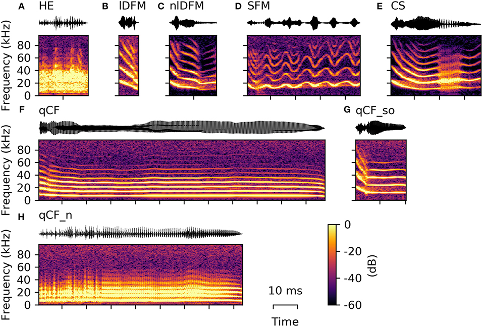
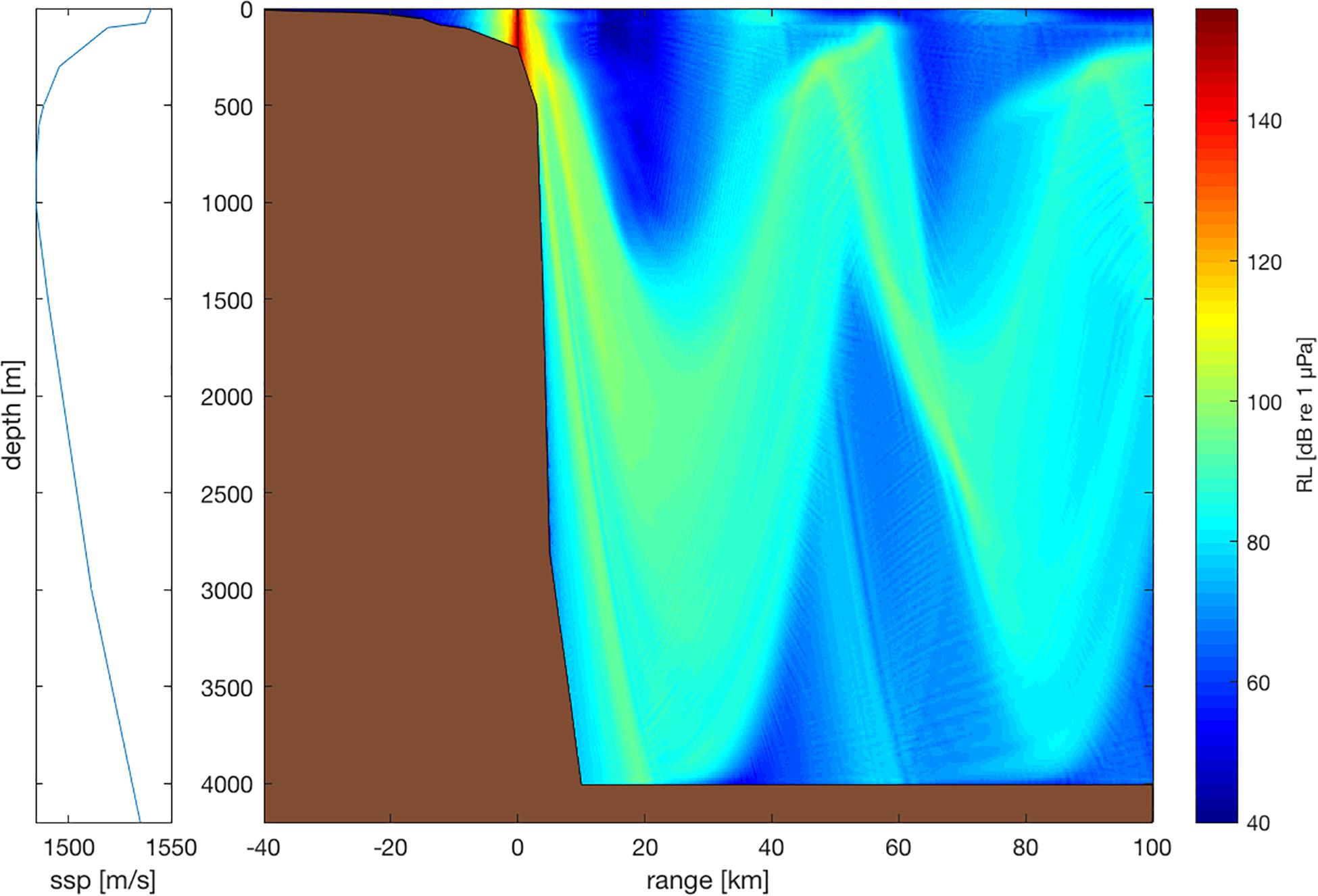
Cite this chapter
Schoeman, R.P., Erbe, C., Pavan, G., Righini, R., Thomas, J.A. (2022). Analysis of Soundscapes as an Ecological Tool. In: Erbe, C., Thomas, J.A. (eds) Exploring Animal Behavior Through Sound: Volume 1. Springer, Cham. https://doi.org/10.1007/978-3-030-97540-1_7
Download citation
DOI: https://doi.org/10.1007/978-3-030-97540-1_7
Published:
Publisher Name: Springer, Cham
Print ISBN: 978-3-030-97538-8
Online ISBN: 978-3-030-97540-1
eBook Packages: Biomedical and Life SciencesBiomedical and Life Sciences (R0)