
You have full access to this open access chapter, Download chapter PDF
In this section, we prove that local minimizers of the functional \(\mathcal F_\Lambda \) do exist (Proposition 2.1) and we give several important examples of local minimizers that can be computed explicitly (Proposition 2.10, Lemmas 2.15 and 2.16).
Let Λ > 0, \(D \subset \mathbb {R}^d\) be a bounded open set and the function g ∈ H 1(D) be fixed and such that g ≥ 0 in D. Then, there exists a solution to the variational problem
Moreover, every solution u of (2.1) has the following properties:
-
(i)
u is non-negative in D;
-
(ii)
u is locally bounded in D;
-
(iii)
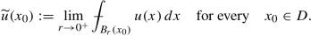
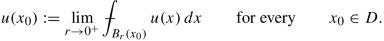
there is a function \(\tilde u:D\to \mathbb {R}\) such that \(\tilde u\ge 0\) and \(\tilde u=u\) almost everywhere in D and
$$\displaystyle \begin{aligned} \tilde u(x_0)=\lim_{r\to 0}\frac 1{|B_r|}\int_{B_r(x_0)}\tilde u(x)\,dx\qquad \mathit{\text{for every}}\qquad x_0\in D. \end{aligned}$$
From now on, we will identify any solution u of (2.1) with its representative \(\tilde u\); for the sake of simplicity, we will always write u instead of \(\tilde u\).
The rest of the section is organized as follows. In Sect. 2.1 we discuss some of the properties (scaling and truncation) of the function \(\mathcal F_\Lambda \). Section 2.2 is dedicated to the proof of Proposition 2.1. In Sects. 2.3 and 2.4, we discuss several examples of local minimizers, which we will find application in the next sections.
2.1 Properties of the Functional \(\mathcal F\)
In this section, we discuss several basic properties of the functional
We give the precise statements in Lemmas 2.3, 2.4 and 2.5.
Lemma 2.3 (Scaling)
Let \(\Omega \subset \mathbb {R}^d\) be an open set and u ∈ H 1( Ω).
-
(a)
Let \(x_0\in \mathbb {R}\) , r > 0 and
$$\displaystyle \begin{aligned} u_{x_0,r}(x):=\frac 1ru(x_0+rx)\qquad \mathit{\text{and}}\qquad \Omega_{x_0,r}=\left\{x=\frac{y-x_0}{r}\in\mathbb{R} :\ y\in \Omega\right\}. \end{aligned}$$Then \(u_{x_0,r}\in H^1(\Omega _{x_0,r})\) and
$$\displaystyle \begin{aligned} \mathcal F_\Lambda(u_{x_0,r},\Omega_{x_0,r})=r^{-d}\,\mathcal F_\Lambda(u,\Omega). \end{aligned}$$In particular, if u is a minimizer of \(\mathcal F_\Lambda \) in Ω, then \(u_{x_0,r}\) is a minimizer of \(\mathcal F_\Lambda \) in \(\Omega _{x_0,r}\).
-
(b)
For every t > 0, we have
$$\displaystyle \begin{aligned} \mathcal F_{t^{2}\Lambda}(tu,\Omega)=t^2\,\mathcal F_\Lambda(u,\Omega). \end{aligned}$$In particular, if u is a minimizer of \(\mathcal F_\Lambda \) in Ω, then tu is a minimizer of \(\mathcal F_{t^{2}\Lambda }\) in Ω.
Proof
The proof is a straightforward computation. □
Lemma 2.4 (Truncation)
Let \(\Omega \subset \mathbb {R}^d\) be an open set and u ∈ H 1( Ω). Then,
Moreover, for every t ≥ 0, we have
Proof
The proof follows by the definition of \(\mathcal F\) and the identities

□
Lemma 2.5 (Comparison)
Let \(\Omega \subset \mathbb {R}^d\) be an open set and u, v ∈ H 1( Ω) be two given functions. Then we have
Proof
The proof is a straightforward computation. In fact, we have
which concludes the proof. □
2.2 Proof of Proposition 2.1
In this section we prove Proposition 2.1. We will first show that the minimizers of \(\mathcal F_\Lambda \) are subharmonic functions (Lemmas 2.6 and 2.7) and then we will deduce the claim (iii) of Proposition 2.1 (see Remark 2.2). At the end of this section, we will complete the proof of Proposition 2.1 by proving that there is a solution to the variational problem (2.1). Finally, in Lemma 2.9, we discuss the definition of the free boundary, which can be (equivalently) defined both as the topological boundary of the representative \(\tilde u\) (of the function u ∈ H 1(D)) defined in Proposition 2.1 and as the measure-theoretic boundary of Ωu, which does not depend on the representative of u and is defined as the set of points x 0 ∈ D for which

Lemma 2.6 (The Minimizers of \(\mathcal F_\Lambda \) Are Subharmonic Functions)
Let \(D\subset \mathbb {R}^d\) be a bounded open set and the non-negative function u ∈ H 1(D) be a minimizer of \(\mathcal F_\Lambda \) in D. Then u is subharmonic, Δu ≥ 0, on D in sense of distributions:
Proof
Let \(\varphi \in C^\infty _c(D)\) be a given non-negative function. Suppose that t ≥ 0 and v = u − tφ. Then we have that v + ≤ u. In particular, integrating on the support of φ we have
This implies that
and the claim follows by taking the (right) derivative at t = 0. □
There is also a more general result, which applies not only to minimizers, but also to generic non-negative functions, which are harmonic where they are strictly positive. The proof can also be found in the book of Henrot and Pierre [36].
Lemma 2.7 (The Minimizers of \(\mathcal F_\Lambda \) Are Subharmonic Functions II)
Let \(D\subset \mathbb {R}^d\) be a bounded open set and the non-negative function u ∈ H 1(D) be harmonic in the set Ω u := {u > 0}, that is

Then u is subharmonic, Δu ≥ 0, on D in sense of distributions.
Proof
Let \(\phi \in C^\infty _c(D)\) be a given non-negative function and let \(p_{\varepsilon }:\mathbb {R}\to \mathbb {R}\) be given by
Since u t := u + t p ε(u)ϕ is a competitor for u and for \(t\in \mathbb {R}\) small enough
we have that for t small enough
which gives
where the last inequality is due to the fact that p
ε is increasing. Now since p
ε(u) converges to  , as ε → 0, we get that
which concludes the proof. □
Remark 2.8 (Pointwise Definition of a Subharmonic Function)
Let D be an open set and u ∈ H 1(D) be a subharmonic function. Then, for every x 0 ∈ D, we have that

As a consequence of (2.2), we obtain that:
-
u is locally bounded, \(u\in L^\infty _{loc}(D)\);
-
we define \(\tilde u:D\to \mathbb {R}\) as

Proof of Proposition 2.1
We first prove that a solution exists. Let u n ∈ H 1(D) be a minimizing sequence such that \(u_n-g\in H^1_0(D)\) and
By Lemma 2.4 we may assume that, for every n ≥ 1, u n ≥ 0 on D. For simplicity, we assume that d > 2 (the case d = 2 is analogous) and we set \(\displaystyle 2^*=\frac {2d}{d-2}\). Then, we have
Now, we estimate,
which implies that the sequence u n is uniformly bounded in H 1(D). Then, up to a subsequence, we may assume that u n converges weakly in H 1(D) and strongly in L 2(D) to a function u ∈ H 1(D). Now, the semi-continuity of the H 1 norm (with respect to the weak H 1 convergence) gives that
On the other hand, passing again to a subsequence, we get that u n converges pointwise almost everywhere to u. This implies that

and so,
which finally gives that
and so, u is a solution to (2.1). Now, we notice that Lemma 2.4 implies that u ≥ 0 on D. Lemma 2.6 and Remark 2.8 give the claims (ii) and (iii). □
We conclude this subsection with the following lemma, where we show that the set Ωu has a topological boundary that coincides with the measure theoretic one.
Lemma 2.9 (Topological and Measure Theoretic Free Boundaries)
Let \(D\subset \mathbb {R}^d\) be a bounded open set and u be a local minimizer of \(\mathcal F_\Lambda \) in the open set \(D\subset \mathbb {R}^d\) or, more generally, let \(u:D\to \mathbb {R}\) , u ∈ H 1(D), be a non-negative function satisfying
-
(a)
u is harmonic in Ω u = {u > 0} in the sense that
-
(b)
u is defined everywhere in D and


Then, the topological boundary of Ω u coincides with the measure-theoretic one:
Proof
We first notice that the following inclusion holds :
In order to prove the opposite inclusion we show that
-
(i)
if |B r ∩{u = 0}| = 0, then u is harmonic in B r and B r ∩{u = 0} = ∅.
-
(ii)
if |B r ∩{u > 0}| = 0, then u = 0 in B r, i.e. B r ∩{u > 0} = ∅.
In order to prove (i) we notice that u is necessarily harmonic in B r, since otherwise we can contradict the minimality of u by replacing it with the harmonic function with the same boundary values. By the strong maximum principle, u is strictly positive in B r. The proof of (ii) follows directly from (b). □
2.3 Half-Plane Solutions
The so-called half-plane solutions (see Fig. 2.1)
play a fundamental role in the free boundary regularity theory. In fact, in the next sections we will show that if a local minimizer u is close to a half-plane solution (at some, possibly very small, scale), then the free boundary is C 1, α regular; then, we will also prove that at almost-every free boundary point the solution u coincides with a half-plane solution at order 1.

A half-plane solution
In this subsection, we make a first step in this direction and we prove that the half-plane solutions are global minimizers. This result is usually omitted in the literature since it is implicitly contained in the fact that the blow-up limits at the points of the reduced free boundary (of any local minimizer) are indeed half-plane solutions (we will prove this fact later, in Lemma 6.11). The main result of this subsection is the following.
Proposition 2.10 (The Half-Plane Solutions Are Local Minimizers)
Let \(\nu \in \mathbb {R}^d\) be a unit vector. Then the function \(H_\nu (x)=\sqrt {\Lambda }\,(\nu \cdot x)_+\) is a global minimizer of \(\mathcal F_\Lambda \).
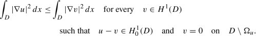
Definition 2.11 (Local Minimizers)
Let D be an open set in \(\mathbb {R}^d\). We say that the function \(u:D\to \mathbb {R}\) is a local minimizer of \(\mathcal F_\Lambda \) in D, if \(u\in H^1_{loc}(D)\), u ≥ 0, and for any bounded open set Ω such that \(\overline \Omega \subset D\), we have
Definition 2.12 (Global Minimizers)
We say that the function \(u:\mathbb {R}^d\to \mathbb {R}\) is a global minimizer of \(\mathcal F_\Lambda \), if u is non-negative on \(\mathbb {R}^d\), \(u\in H^1_{loc}(\mathbb {R}^d)\) and u is a local minimizer of \(\mathcal F_\Lambda \) in \(\mathbb {R}^d\).
In order to prove the minimality of the half-plane solutions, we will need the following lemma. We notice that it is useful also in other contexts. For instance, it allows to prove that the solutions of (2.1) are bounded.
Lemma 2.13
Let \(D\subset \mathbb {R}^d\) be a bounded smooth open set or \(D=\mathbb {R}^d\) . Let \(x_0\in \mathbb {R}^d\) be a given point, \(\nu \in \mathbb {R}^d\) be a unit vector and let
Suppose that u ∈ H 1(D) is a non-negative function such that
Then
with an equality if and only if u = u ∧ v.
In particular, if u is a solution to (2.1), then u has bounded support. Precisely, u = 0 outside the set conv(D) + B 1 , where conv(D) is the convex hull of D.
Proof
Without loss of generality we can suppose that ν = e d and x 0 = 0. For the sake of simplicity, we set H + = {x d > 0} and H − = {x d < 0}. Then
where (in the case when D is bounded) we assume that u is extended by zero on  . By the fact that \(v(x)=\Lambda x_d^+\) is harmonic on {x
d > 0}, we get that
. By the fact that \(v(x)=\Lambda x_d^+\) is harmonic on {x
d > 0}, we get that
We recall that for every u ∈ H 1({x d < 0}) we have the inequalityFootnote 1
where the equality holds, if and only if, u ≡ 0 on {x d < 0}. Thus, we obtain
where the last inequality is an equality if and only if u ≤ v on \(\mathbb {R}^d\). □
Proof of Proposition 2.10
Without loss of generality we may suppose that ν = e d and set
Suppose that R > 0 and \(u\in H^1_{loc}(\mathbb {R}^d)\) is a non-negative function such that \(u-h\in H^1_0(B_R)\). It is sufficient to prove that \(\mathcal F_\Lambda (h,B_R)\le \mathcal F_\Lambda (u,B_R)\). By Lemma 2.13 we have that
Thus, we may suppose that u ≤ h. Since h is harmonic in {x d > 0} we get that
where the last equality is due to the fact that
This concludes the proof. □
2.4 Radial Solutions
In this subsection, we give two examples of local minimizers, which are radial functions. Despite of being ones of the few non-trivial examples of local minimizers, they will also be useful in the proof (to be precise, in one of the two proofs that we will give) of the fact that the local minimizers satisfy an overdetermined condition on the free boundary in viscosity sense (see Definition 7.6 and Proposition 7.1).
Let D be a bounded open set in \(\mathbb {R}^d\) with smooth boundary. We consider the following variational minimization problem in the exterior domain  .
.
The “interior” version of this problem reads as
We first prove that the problems (2.3) and (2.4) admit solutions.
Lemma 2.14 (Existence of a Solution)
Suppose that D is a bounded open set in \(\mathbb {R}^d\) with smooth boundary. Then the variational problems (2.3) and (2.4) admit solutions.
Proof
We give the proof for (2.3), the case (2.4) being analogous (and easier as it does not require the use of Lemma 2.13). Let u n be a minimizing sequence in \(H^1(\mathbb {R}^d)\). By Lemmas 2.4 and 2.13 we can suppose that 0 ≤ u n ≤ 1 and supp (u n) ⊂ conv(D) + B 1. Now, up to a subsequence, we may suppose that u n converges in \(L^2(\mathbb {R}^d)\) and pointwise almost everywhere to a function \(u\in H^1(\mathbb {R}^d)\). The claim follows by the semicontinuity of \(\mathcal F_\Lambda \). □
In Propositions 2.15 and 2.16, we will prove that, in the special case when the domains D in (2.3) and (2.4) are balls, the solution is unique and can be computed explicitly.
Proposition 2.15 (Optimal Exterior Domains)
Let the domain D in \(\mathbb {R}^d\) be the ball B r . Then, there is a unique solution u r of (2.3). Moreover, for every r, there is a radius R > r, uniquely determined by r and d, such that u r is given by

where h r is a radial harmonic function (as on Fig. 2.2). Precisely, h r is given by

An exterior radial solution
Moreover, the radius R and the function u r satisfy the following properties:
-
(i)
The radius R = R(r) is a continuous function of r such that
$$\displaystyle \begin{gathered} r<R<r+1\\ \mathit{and}\\ \displaystyle\lim_{r\to+\infty}|R(r)-(r+1)|=0. \end{gathered} $$ -
(ii)
The gradient of h r is given by
$$\displaystyle \begin{aligned} |\nabla h_r|(x)=\left(|x|/R\right)^{1-d}. \end{aligned}$$
Proof
We first notice that taking the Schwartz symmetrization u ∗ of any function u we get that \(\mathcal F_1(u^\ast ,\mathbb {R}^d)\le \mathcal F_1(u,\mathbb {R}^d)\). Thus, there is a minimizer of \(\mathcal F_1\) which is a radial function. We first show that there is a unique radial function that minimizes of \(\mathcal F_1\) in the class of radial functions.
Let d ≥ 3. For every 0 < r < R, consider the function
Since u
r,R is the unique harmonic function in  , we get that the minimizer of \(\mathcal F_1\) among the radial functions is necessarily given by a function of the form u
r,R. We calculate the energy
, we get that the minimizer of \(\mathcal F_1\) among the radial functions is necessarily given by a function of the form u
r,R. We calculate the energy

We notice that the function \(f(R):=\displaystyle \frac {d(d-2)}{r^{2-d}-R^{2-d}}+ R^d\) is strictly convex and
Thus, there is a unique radius R > r that minimizes f. We denote this radius by R ∗. Notice that, since f′(R ∗) = 0, we have
Let d = 2. For every 0 < r < R, consider the function
As in the case d ≥ 3, we calculate the energy

As in the case d > 2, there is a unique R ∗ > r that minimizes the function \(R\mapsto \mathcal F(u_{r,R})\). Moreover, R ∗ is such that
We notice that the claims (i) and (ii) follow by (2.5) and (2.6).
We now prove that the functions \(u_{r,R_\ast }\) are the unique minimizers of \(\mathcal F_1\) among all admissible functions. Indeed, consider any minimizer u of \(\mathcal F_1\) and suppose that it is not radial. We notice that the symmetrized function u ∗ is also a solution. Since it is radial, we get that \(u^\ast =u_{r,R^\ast _d}\) and in particular \(|\{u>0\}|=|B_{R_\ast }|\). By Lemma 2.5, the functions v = u ∧ u ∗ and V = u ∨ u ∗ are also minimizers of \(\mathcal F\). If u is not radial, then we have \(|\{v>0\}|\neq |B_{R_\ast }|\) or \(|\{v>0\}|\neq |B_{R_\ast }|\). On the other hand the symmetrized function v ∗ and V ∗ are also solutions and so, we must have v ∗ = V ∗ = u ∗ and in particular \(|\{v>0\}|=|\{V>0\}|=|B_{R_\ast }|\), which is in contradiction with the assumption that u is not radially symmetric. □
Proposition 2.16 (Optimal Interior Domains)
Let the domain D in \(\mathbb {R}^d\) be the ball B R . Then, there is a dimensional constant C d > 0 such that, for every R > C d , there is a unique solution u R of (2.4). Moreover, u R is radially symmetric and has the following properties:

where h R is a radially symmetric harmonic function (see Fig. 2.3). Precisely,

An interior radial solution
where the radius r depends on R and d and has the following properties:
-
(i)
The radius r = r(R) is a continuous function of R such that
$$\displaystyle \begin{aligned} \displaystyle\lim_{R\to+\infty}|r(R)-(R-1)|=0. \end{aligned}$$ -
(ii)
The gradient of h R is given by
$$\displaystyle \begin{aligned} |\nabla h_R|(x)=\left({|x|/r}\right)^{1-d}. \end{aligned}$$
Proof
As in the proof of Lemma 2.15, we start by noticing that for every function u, there is a radially symmetric function u ∗ with lower energy. In fact, it is sufficient to consider the function v = 1 − u and its Schwartz symmetrization v ∗. We define u ∗ as u ∗ := 1 − v ∗ and we notice that
Thus, there exists a radially symmetric minimizer u ∗ of \(\mathcal F\). Now, since u ∗ is harmonic in {u ∗ > 0}, it should be of the form u ∗ = u r,R, where u r,R is given by (2.7) for some radius r < R. Now, for any r ∈ (0, R), the energy of u r,R is given by

Consider the function
It is easy to check that,
Moreover, for R large enough, f(R∕2) < 0. We now calculate
Thus, f′(r) = 0 if and only if
Now, the equation g(r) = 0 has at most two solutions and we have that
On the other hand, for R large enough, we have
Thus, the equation g(r) = 0 has exactly two solutions:
Now, let M d be the minimum of f in the interval [0, d − 1]. For R large enough, we have
Thus, there is a unique r ∈ (0, R) that minimizes f in (0, R). Moreover, R − 2 < r < R. Moreover, the claim (i) follows from the fact that, for every ε > 0, there is R ε > 0 such that if R > R ε, then
This implies that R − (1 + ε) ≤ r(R) ≤ R − (1 − ε), which is precisely (i).
Let now d = 2. For every r ∈ (0, R), consider the function u r,R given by (2.7) for some r > 0. We calculate the energy

Next, we define
we calculate
and we set
As above, g can have at most two zeros in the interval (0, R). Moreover, g(0) = g(R) = 1 and for R large enough, we have
Thus, the two zeros of g are in the intervals (0, 1) and (R − 2, R), respectively. Now, for R large enough, we have
Thus, for large enough R, there is a unique r that minimizes f in (0, R) and R − 2 < r < R. The claim (i) follows as in the case d > 2. The claim (ii) is immediate and follows from the equation g(r) = 0. The uniqueness of the solution now follows as in Lemma 2.15. □
Notes
- 1.
Indeed, if \(f:\mathbb {R}\to \mathbb {R}^+\) is a Sobolev function such that f(a) = 0 for some a < 0, then we have
$$\displaystyle \begin{aligned} f(0)=\int_{a}^0 f'(t)\,dt\le \big|\{f\neq 0\}\cap\{a\le t\le 0\}\big|{}^{\frac 12}\left(\int_{a}^0 |f'(t)|{}^2\,dt\right)^{\frac 12}\le \frac 12\left(\big|\{f\neq 0\}\cap\{t\le 0\}\big|+\int_{a}^0 |f'(t)|{}^2\,dt\right). \end{aligned}$$
References
A. Henrot, M. Pierre, Variation et Optimisation de Formes. Une Analyse Géométrique. Mathématiques & Applications, vol. 48 (Springer, Berlin, 2005)
Author information
Authors and Affiliations
Rights and permissions
Open Access This chapter is licensed under the terms of the Creative Commons Attribution 4.0 International License (http://creativecommons.org/licenses/by/4.0/), which permits use, sharing, adaptation, distribution and reproduction in any medium or format, as long as you give appropriate credit to the original author(s) and the source, provide a link to the Creative Commons license and indicate if changes were made.
The images or other third party material in this chapter are included in the chapter's Creative Commons license, unless indicated otherwise in a credit line to the material. If material is not included in the chapter's Creative Commons license and your intended use is not permitted by statutory regulation or exceeds the permitted use, you will need to obtain permission directly from the copyright holder.
Copyright information
© 2023 The Author(s)
About this chapter

Cite this chapter
Velichkov, B. (2023). Existence of Solutions, Qualitative Properties and Examples. In: Regularity of the One-phase Free Boundaries. Lecture Notes of the Unione Matematica Italiana, vol 28. Springer, Cham. https://doi.org/10.1007/978-3-031-13238-4_2
Download citation
DOI: https://doi.org/10.1007/978-3-031-13238-4_2
Published:
Publisher Name: Springer, Cham
Print ISBN: 978-3-031-13237-7
Online ISBN: 978-3-031-13238-4
eBook Packages: Mathematics and StatisticsMathematics and Statistics (R0)