Lipschitz Continuity of the Minimizers

Abstract

In this section, we will prove that the local minimizers of $\mathcal F_\Lambda$ are Lipschitz continuous. Our main result is the following.

In this section, we will prove that the local minimizers of $\mathcal F_\Lambda$ are Lipschitz continuous. Our main result is the following.

FormalPara Theorem 3.1

Let $D\subset \mathbb {R}^d$ be an open set and $u\in H^1_{loc}(D)$ . Suppose that u is a local minimizer of $\mathcal F_\Lambda$ in D. Then, u is locally Lipschitz continuous in D.

Theorem 3.1 is a consequence of the more general Theorem 3.2, which can be applied not only to minimizers of $\mathcal F_\Lambda$ (we will need this result for the proofs of Theorems 1.2, 1.4 and 1.10), but also to the case of minimizers for the problem with a measure constraint (Theorem 1.9); we notice that we will be able to apply Theorem 3.2 to (1.6) only after proving that an outwards minimality property of the type (3.1) holds at very small scale (see Sect. 11.5).

FormalPara Theorem 3.2

Let D be a bounded open set in $\mathbb {R}^d$ and u ∈ H ¹(D) be a non-negative function satisfying the following minimality condition:

$$\displaystyle \begin{aligned} \mathcal F_\Lambda(u,D)\le \mathcal F_\Lambda(v,D)\quad & \mathit{\text{for every}}\quad v\in H^1(D)\quad \mathit{\text{such that}}\notag \\ & \qquad u-v\in H^1_0(D)\quad \mathit{\text{and}}\quad \Omega_u\subset\Omega_v.{} \end{aligned} $$

(3.1)

Then, u is locally Lipschitz continuous in D.

The outwards minimality condition appeared recently in [9] in the context of a shape optimization problem, which can be reduced to a free boundary problem for vector-valued functions (see [41]). This property proved to be very useful only in the context of other free boundary and shape optimization problems as, for instance, the ones involving functionals depending on the perimeter of the set (see [21] and [22]). In the case of $\mathcal F_\Lambda$ the outwards minimality condition (3.1) can also be expressed in a different way. We give the precise statement in the following lemma.

FormalPara Lemma 3.3

Let D be a bounded open set in $\mathbb {R}^d$ and u ∈ H ¹(D) be a given non-negative function. Then the following are equivalent:

• (i) u satisfies the minimality condition (3.1);

• (ii) u is harmonic in Ω _u in the following sense:

  

  (3.2)

  and satisfies the minimality condition

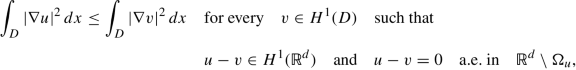
  $$\displaystyle \begin{aligned} \mathcal F_\Lambda(u,D)\le \mathcal F_\Lambda(v,D)\quad & \mathit{\text{for every}}\quad v\in H^1(D)\quad \mathit{\text{such that}}\notag\\ & \qquad u-v\in H^1_0(D)\quad \mathit{\text{and}}\quad u\le v\quad \mathit{\text{in}}\quad D.{}\end{aligned} $$

  (3.3)

FormalPara Remark 3.4 (On the Sign of the Test Functions in (3.1), (3.2) and (3.3))

Since u is non-negative in D, we may suppose that the test functions v in (3.1), (3.2) and (3.3) are all non-negative.

FormalPara Proof of Lemma 3.3

The fact that (3.1) implies (3.2) and (3.3) is trivial. Suppose now that u satisfies both (3.2) and (3.3) and let v ∈ H ¹(D) be a non-negative function such that $u-v\in H^1_0(D)$ and Ω_u ⊂ Ω_v. Then consider the test functions u ∧ v and u ∨ v. Since u ∧ v = 0 outside Ω_u, by (3.2), we have that

$$\displaystyle \begin{aligned} \int_D|\nabla u|{}^2\,dx\le \int_D|\nabla (u\wedge v)|{}^2\,dx. \end{aligned}$$

On the other hand, since u ∨ v ≥ u, (3.3) implies that

$$\displaystyle \begin{aligned} \int_D|\nabla u|{}^2\,dx+\Lambda |\Omega_u|\le \int_D|\nabla (u\vee v)|{}^2\,dx+\Lambda |\Omega_{u\vee v}|. \end{aligned}$$

Summing up the two inequalities, we get

$$\displaystyle \begin{aligned} 2\int_D|\nabla u|{}^2\,dx+\Lambda |\Omega_u|& \le \int_D|\nabla (u\wedge v)|{}^2\,dx+\int_D|\nabla (u\vee v)|{}^2\,dx+\Lambda |\Omega_{u\vee v}|\\ & = \int_D|\nabla u|{}^2\,dx+\int_D|\nabla v|{}^2\,dx+\Lambda |\Omega_{v}|, \end{aligned} $$

which is precisely (3.1). □

We will give three different proofs of Theorem 3.2, but in each one of them, the conclusion (the Lipschitz continuity of u) will be a consequence of the following estimate on the growth of the function u at the free boundary

(3.4)

where r ₀ > 0 and C > 0 are universal constants depending on the distance to the boundary ∂D. We give the precise statement in the following lemma.

FormalPara Lemma 3.5

Suppose that u ∈ H ¹(D) is a non-negative function such that:

• u is harmonic in the interior of the set Ω _u := {u > 0};

• u satisfies the inequality (3.4) with constants C and r ₀ uniformly in D.

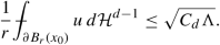
Then the set Ω _u is open and the function u is locally Lipschitz continuous in D. Precisely, the gradient of u can be estimated as

$$\displaystyle \begin{aligned} \|\nabla u\|{}_{L^\infty(D_\delta)}\le C_d\left(C+\frac{\|u\|{}_{L^1(D_{\frac\delta2})}}{\delta^{d+1}}\right)\qquad \mathit{\text{for every}}\qquad 0<\delta<r_0, \end{aligned}$$

where C _d is a dimensional constant and, for r > 0, we use the notation

$$\displaystyle \begin{aligned} D_r:=\big\{x\in D\ :\ \mathit{\text{dist}}\,(x,\partial D)>r\big\}. \end{aligned}$$

FormalPara Proof

Suppose that x ₀ ∈ D ∩ ∂ Ω_u. Passing to the limit as r → 0 the estimate (3.4) we obtain that u(x ₀) = 0. Thus Ω_u ∩ ∂ Ω_u = ∅ and so Ω_u is open.

Let now x ₀ ∈ D _δ. We consider two cases.

• If dist(x ₀, ∂ Ω_u) ≥ δ∕4, then u is harmonic in the ball B _δ∕4(x ₀) and so, by the gradient estimate (see for example [30]) we have

  $$\displaystyle \begin{aligned} |\nabla u(x_0)|\le \frac{C_d}{\delta^{d+1}}\int_{B_\delta(x_0)}u\,dx, \end{aligned}$$

  where C _d is a dimensional constant.

• If dist(x ₀, ∂ Ω_u) < δ∕4, then we suppose that the distance to the free boundary is realized by some y ₀ ∈ ∂ Ω_u and we set

  $$\displaystyle \begin{aligned} r=\mbox{dist}(x_0,\partial\Omega_u)=|x_0-y_0|. \end{aligned}$$

  Since u is harmonic in B _r(x ₀), we can again apply the gradient estimate obtaining

  $$\displaystyle \begin{aligned} |\nabla u(x_0)|& \le \frac{C_d}{r^{d+1}}\int_{B_r(x_0)}u\,dx\le \frac{C_d}{r^{d+1}}\int_{B_{2r}(y_0)}u\,dx\le C_d\, C, \end{aligned} $$

  where the second inequality follows by the positivity of u and the inclusion B _r(x ₀) ⊂ B _2r(y ₀). The last inequality is simply a consequence of (3.4) and the fact that

  $$\displaystyle \begin{aligned} \int_{B_{2r}(y_0)}u\,dx=\int_0^{2r}\,ds\int_{\partial B_s(y_0)}u\,d\mathcal{H}^{d-1}. \end{aligned}$$

□

FormalPara Remark 3.6 (An Alternative Statement of (3.4))

We notice that (3.4) is a consequence of the following inequality

(3.5)

This is trivial if we knew a priori that u is continuous, but is true also in general. Indeed, by Lemma 2.9, we have that

$$\displaystyle \begin{aligned} \partial\Omega_u=\Big\{x_0\in D\ :\ 0<|\Omega_u\cap B_r(x_0)|<|B_r|\quad \text{for every}\quad r>0\Big\}. \end{aligned}$$

Thus, every point x ₀ ∈ ∂ Ω_u can be obtained as limit of points x _n ∈{u = 0}, for which the estimate (3.5) does hold. The claim follows by the continuity of the function

for every fixed r > 0, which is due to the fact that u ∈ H ¹(D).

The rest of this section is dedicated to the proof of (3.4) in the hypotheses of Theorem 3.2. In the next three subsections we will give three different proofs of this fact.

• Section 3.1 . The Alt-Caffarelli proof of the Lipschitz continuity.

  In this section we present the original proof proposed by Alt and Caffarelli (see [3]), which we divide in two steps (Lemmas 3.7 and 3.8). This entire section comes directly from [51] and we report it here for the sake of completeness.

• Section 3.2 . The Laplacian estimate.

  In this section we give a proof, which is inspired from the proof of the Lipschitz continuity of the solution to the two-phase problem, which was given by Alt, Caffarelli and Friedman in [4]. In our case there is only one phase (that is, the solution u is positive), so we do not make use of the two-phase monotonicity formula of Alt-Caffarelli-Friedman, which significantly simplifies the proof. This approach can be used also in other situations, for instance, for functionals involving elliptic operators (in divergence form) with non-constant coefficients (see [46]).

• Section 3.3 . The Danielli-Petrosyan approach.

  This last subsection is dedicated to the method proposed by Danielli and Petrosyan in [18] in the context of non-linear operators. It consists of two steps. The first one is to show that u is Hölder continuous. This part of the argument is very general and is based on classical regularity estimates for (almost-)minimizers of variational problems. In the second step of the proof, the Lipschitz continuity is obtained by absurd and the result of the first step is used to assure the convergence of the sequence of minimizers produced by contradiction. This type of argument (proving a weaker estimate and then obtaining the main result by contradiction) will be used also in Chap. 8, this time to obtain the regularity of the free boundary.

3.1 The Alt-Caffarelli’s Proof of the Lipschitz Continuity

This subsection contains the original argument proposed by Alt and Caffarelli in [3]. The main steps of the proof are the following:

• Comparing the energy $\mathcal F_\Lambda (u,B_r(x_0))$ of u in the ball B _r(x ₀) with the one of the harmonic extension h of u in B _r(x ₀) we get

  $$\displaystyle \begin{aligned} \int_{B_r(x_0)}|\nabla (u-h)|{}^2\,dx\le \Lambda \big|\{u=0\}\cap B_r(x_0)\big|. \end{aligned}$$

• It is now sufficient to estimate from below the right-hand side of the above inequality. In Lemma 3.7 we will prove that

  

• If x ₀ ∈ Ω_u, then |{u = 0}∩ B _r(x ₀)| ≠ 0. Combining the two inequalities we get

  

We now give the details of the proof sketched above. The key ingredient is the following trace-type inequality (Lemma 3.7), which is implicitly contained in the proof of the Lipschitz continuity given in [3] (and can also be found in [51]) and is an interesting result by itself.

Lemma 3.7

For every u ∈ H ¹(B _r) we have the following estimate:

(3.6)

where:

• C _d is a constant that depends only on the dimension d;

• h is the harmonic replacement of u in B _r , that is, the harmonic function in B _r such that u = h on ∂B _r.

Proof

We report here the proof for the sake of completeness, and refer the reader to [3, Lemma 3.2 ]. We note that it is sufficient to prove the result in the case u ≥ 0. Let v ∈ H ¹(B _r) be the solution of the problem

$$\displaystyle \begin{aligned} \min\left\{\int_{B_r}|\nabla v|{}^2\,dx:\ u-v\in H^1_0(B_r),\ v\ge u\right\}. \end{aligned}$$

Notice that v is super-harmonic on B _r and harmonic on the set {v > u}.

For each |z|≤ 1∕2, we consider the functions u _z and v _z defined on B _r as

$$\displaystyle \begin{aligned} u_z(x):=u\big((r-|x|)z+x\big)\qquad \mbox{and}\qquad v_z(x):=v\big((r-|x|)z+x\big). \end{aligned}$$

Note that both u _z and v _z still belong to H ¹(B _r) and that their gradients are controlled from above and below by the gradients of u and v. We call S _z the set of all |ξ| = 1 such that the set $\displaystyle \big \{\rho :\frac {r}{8}\leq \rho \leq r,\ u_z(\rho \xi )=0\big \}$ is not empty. For ξ ∈ S _z we define

$$\displaystyle \begin{aligned} r_{\xi}=\inf\Big\{\rho:\frac{r}{8}\leq\rho\leq r,\ u_z(\rho\xi)=0\Big\}. \end{aligned}$$

For almost all ξ ∈ S ^d−1 (and then for almost all ξ ∈ S _z), the functions ρ↦∇u _z(ρξ) and ρ↦∇v _z(ρξ) are square integrable. For those ξ, one can suppose that the equation

$$\displaystyle \begin{aligned} \big((u_z(\rho_2\xi)-v_z(\rho_2\xi)\big)-\big(u_z(\rho_1\xi)-v_z(\rho_1\xi)\big)=\int_{\rho_1}^{\rho_2}\xi\cdot\nabla\big(u_z(\rho\xi)-v_z(\rho\xi)\big)\, d\rho, \end{aligned}$$

holds for all ρ ₁, ρ ₂ ∈ [0, r]. Moreover, we have the estimate

$$\displaystyle \begin{aligned} v_z(r_{\xi}\xi)=\int_{r_{\xi}}^{r}\xi\cdot\nabla (v_z-u_z)(\rho\xi)\, d\rho\leq\sqrt{r-r_{\xi}}\left(\int_{r_{\xi}}^r|\nabla (v_z-u_z)(\rho\xi)|{}^2\,d\rho\right)^{1/2}. \end{aligned}$$

Since v is superharmonic we have that, by the Poisson’s integral formula,

where h is the harmonic function such that h = u(= v) on ∂B _r. Taking

$$\displaystyle \begin{aligned} x=(r-r_{\xi})z+r_{\xi}\xi, \end{aligned}$$

we have

Combining the two inequalities, we have

Integrating over ξ ∈ S _z ⊂ S ^d−1, we obtain the inequality

and, by the estimate that r∕8 ≤ r _ξ ≤ r, we have

Integrating over z, we obtain (3.6). □

Lemma 3.8

Suppose that $u\in H^1_{loc}(D)$ be a local minimizer of $\mathcal F_\Lambda$ in the open set $D\subset \mathbb {R}^d$ . Then for every ball $\overline B_r(x_0)\subset D$ we have

In particular, if x ₀ ∈ ∂ Ω _u , then

Proof

Suppose that x ₀ = 0. Let h ∈ H ¹(B _r) be the harmonic function in B _r such that h = u on ∂B _r. By the optimality of u we get

$$\displaystyle \begin{aligned} {} \begin{array}{ll} \displaystyle \int_{B_r}|\nabla u|{}^2\,dx+\Lambda\big|\{u>0\}\cap B_r\big|\le \int_{B_r}|\nabla h|{}^2\,dx+\Lambda|B_r|. \end{array} \end{aligned}$$

Now using (3.6) and the fact that

$$\displaystyle \begin{aligned} \int_{B_r}|\nabla (u-h)|{}^2\,dx=\int_{B_r}\Big(|\nabla u|{}^2-|\nabla h|{}^2\Big)\,dx\le \Lambda|\{u=0\}\cap B_r|, \end{aligned}$$

we get

which gives the claim. □

3.2 The Laplacian Estimate

In this section, we propose a different approach to the Lipschitz continuity of u. The method comes from the two-phase free boundary theory and, in particular, from the work of Alt-Caffarelli-Friedman [4] and Briançon-Hayouni-Pierre [7]. This argument was also adapted to the vectorial case in [41] and to a one-phase shape optimization problem in [46]. The proof consists of two steps:

• For every local minimizer u of $\mathcal F_1$ we have that Δu is a positive measure. In Lemma 3.9, we prove that the optimality of u implies the estimate

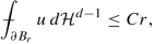
  $$\displaystyle \begin{aligned} \Delta u(B_{r})\le C\,r^{d-1}. \end{aligned}$$

• In Lemma 3.10, we show that the Laplacian estimate and the classical identity

  

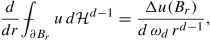
  imply that

  

  which gives the Lipschitz continuity of u by Proposition 3.5.

Lemma 3.9 (The Laplacian Estimate)

Suppose that u is a local minimizer of $\mathcal F_1$ in D. Then, for every ball B _r(x ₀) such that B _2r(x ₀) ⊂ D we have

$$\displaystyle \begin{aligned} \Delta u(B_r(x_0))\le C\,r^{d-1}. \end{aligned}$$

Proof

Without loss of generality we can assume that x ₀ = 0. We now notice that by Lemma 2.6 the distributional Laplacian

$$\displaystyle \begin{aligned} \Delta u (\varphi):=-\int_D\nabla u\cdot\nabla \varphi\,dx\quad \text{for every}\quad \varphi\in C^1_c(D), \end{aligned}$$

is a positive Radon measure. We first prove that

$$\displaystyle \begin{aligned} \Delta u(\varphi)\le C_d\,r^{\frac{d}2}\,\|\nabla \varphi\|{}_{L^2(B_r)}\quad \text{for every}\quad \varphi\in C^\infty_c(B_r)\quad \text{and every}\quad B_r\subset D. \end{aligned} $$

(3.7)

Indeed, for every $\psi \in C^\infty _c(B_r)$, the optimality of u gives

$$\displaystyle \begin{aligned} \int_{B_r}|\nabla u|{}^2\,dx\le \int_{B_r}|\nabla u|{}^2\,dx+\big|\{u>0\}\cap B_r\big|\le \int_{B_r}|\nabla (u+\psi)|{}^2\,dx+ |B_r|. \end{aligned}$$

Developing the gradient on the right-hand side, we get

$$\displaystyle \begin{aligned} -\int_{B_r}\nabla u\cdot\nabla\psi\,dx\le \frac{1}{2}\left(\int_{B_r}|\nabla\psi|{}^2\,dx+\omega_d\,r^d\right). \end{aligned}$$

Setting $\displaystyle \psi =r^{\frac {d}2}\,\|\nabla \varphi \|{ }_{L^2(B_r)}^{-1}\,\varphi$, we get

$$\displaystyle \begin{aligned} -\int_{B_r}\nabla u\cdot\nabla\varphi\,dx\le \frac{1+\omega_d}{2}\,r^{\frac{d}2}\,\|\nabla\varphi\|{}_{L^2(B_r)}, \end{aligned}$$

which is precisely (3.7) with $\displaystyle C_d=\frac {1+\omega _d}{2}$.

Let now $\varphi \in C^\infty _c(B_{2r})$ be such that

$$\displaystyle \begin{aligned} \varphi\ge 0\ \text{on}\ B_{2r},\qquad \varphi=1\ \text{on}\ B_r,\qquad \text{and}\qquad \|\nabla \varphi\|{}_{L^\infty(B_{2r})}\le \frac 2{r}. \end{aligned}$$

Thus, and by the positivity of Δu we have

$$\displaystyle \begin{aligned} \Delta u(B_r)\le \Delta u(\varphi)\le C_d\,(2r)^{\frac{d}2}\,\|\nabla \varphi\|{}_{L^2(B_{2r})}\le Cr^{d-1}. \end{aligned}$$

□

Now the estimate (3.4) follows by the following lemma.

Lemma 3.10

Suppose that u ∈ H ¹(B _R) is a non-negative sub-harmonic function in the ball $B_R\subset \mathbb {R}^d$ such that u(0) = 0. Suppose that there is a constant C > 0 such that

$$\displaystyle \begin{aligned} \Delta u(B_r)\le C\,r^{d-1}\quad \mathit{\text{for every}}\quad 0<r<R. \end{aligned} $$

(3.8)

Then we have

(3.9)

Proof

We first notice that for every smooth u _ε we have

Integrating in r and passing to the limit as ε → 0 we get

Now, using (3.8) we get (3.9). □

3.3 The Danielli-Petrosyan Approach

Finally, in the last section dedicated to the Lipschitz continuity of the minimizers, we present another proof, which is due to Danielli and Petrosyan and was originally carried out in the framework of the p-laplacian (see [18]). In fact, this proof is very close in spirit to the one of the regularity of the free boundary that we will present in Chap. 8. It consists of two steps. The first one is to prove that the local minimizers are Hölder continuous and to find a uniform estimate on their C ^{0, α} norm (see Lemma 3.11, Lemma 3.12 and Proposition 3.13). Then, the Lipschitz continuity (see Proposition 3.15) follows by a contradiction argument, in which the compactness is a consequence of the aforementioned uniform C ^{0, α} estimate.

Lemma 3.11

Suppose that $\Omega \subset \mathbb {R}^d$ is a bounded open set and that the function u ∈ H ¹( Ω) ∩ L ^∞( Ω) is such that:

• (a) u is non-negative and subharmonic in Ω;

• (b) u satisfies the minimality condition (3.3) for some constant Λ > 0.

Then, setting

$$\displaystyle \begin{aligned} {\varepsilon}=\frac 2d\ ,\qquad \alpha=\frac 2{2+d}\qquad \mathit{\text{and}}\qquad C=2^{d+3}|B_1|\left(\Lambda+\|u\|{}_{L^\infty(\Omega)}^2\right), \end{aligned}$$

the following inequality does hold:

$$\displaystyle \begin{aligned} \int_{B_{\rho}(x_0)}|\nabla u|{}^2\, dx\le C\rho^{d-2(1-\alpha)}\quad \mathit{\text{for every}} \ B_\rho(x_0)\subset \Omega\ \mathit{\text{with}} \ \rho\le 2^{-\frac{d+2}{2}}. \end{aligned}$$

Proof

Let $r=\rho ^{\frac {1}{1+{\varepsilon }}}$. Thus we have B _r(x ₀) ⊂ Ω. Without loss of generality we can assume that x ₀ = 0. Let h be the harmonic extension of u in the ball B _r. Then, u ≤ h and, by the optimality of u, we get

$$\displaystyle \begin{aligned} \int_{B_r}|\nabla (u-h)|{}^2\,dx=\int_{B_r}|\nabla u|{}^2\,dx-\int_{B_r}|\nabla h|{}^2\,dx\le \Lambda|B_r|. \end{aligned}$$

Thus, we can estimate the gradient of u as follows

$$\displaystyle \begin{aligned} \int_{B_{r^{1+{\varepsilon}}}}|\nabla u|{}^2\, dx& \le 2\int_{B_{r^{1+{\varepsilon}}}}|\nabla (u-h)|{}^2\,dx+2 \int_{B_{r^{1+{\varepsilon}}}}|\nabla h|{}^2\,dx\\ & \le 2\int_{B_{r}}|\nabla (u-h)|{}^2\,dx+2 \frac{|B_{r^{1+{\varepsilon}}}|}{|B_{\frac{r}2}|} \int_{B_{\frac{r}2}}|\nabla h|{}^2\,dx\\ & \le 2\Lambda |B_r|+2^{d+1}r^{{\varepsilon} d}\int_{B_{\frac{r}2}}|\nabla h|{}^2\,dx\,, \end{aligned} $$

where the second inequality follows by the fact that |∇h|² is subharmonic in B _r and the inequality r ^ε ≤ 1∕2. Now, we use the Caccioppoli inequality

$$\displaystyle \begin{aligned} \int_{B_{\frac{r}2}}|\nabla h|{}^2\,dx\le \int_{B_{r}}|\nabla (h\varphi)|{}^2\,dx= \int_{B_{r}}|\nabla \varphi|{}^2 \,h^2\,dx\le \|\nabla \varphi\|{}_{L^\infty}^2\int_{B_{r}} \,h^2\,dx\le \frac{4|B_r|M^2}{r^2}, \end{aligned}$$

where $M=\|u\|{ }_{L^\infty (D)}\ge \|h\|{ }_{L^\infty (B_r)}$ and φ is given by

$$\displaystyle \begin{aligned} \varphi(x)=0\ \text{ if }\ |x|\ge r,\qquad \varphi(x)=1\ \text{ if }\ |x|\le \frac{r}2,\qquad \varphi(x)=\frac 2r (r-|x|)\ \text{ if }\ \frac{r}2<|x|< r. \end{aligned}$$

Since ρ = r ^1+ε and ε = 2∕d we obtain

$$\displaystyle \begin{aligned} \int_{B_{\rho}}|\nabla u|{}^2\, dx\le 2\Lambda |B_1|\rho^{\frac{d}{1+{\varepsilon}}}+2^{d+3}|B_1|M^2\rho^{d-\frac{2}{1+{\varepsilon}}}\le 2^{d+3}|B_1|\big(\Lambda+M^2\big)\rho^{\frac{d}{1+{\varepsilon}}} \end{aligned}$$

which gives the claim. □

Lemma 3.12 (Morrey)

Suppose that $\Omega \subset \mathbb {R}^d$ , u ∈ H ¹(B _R) and that there are constants C > 0 and α ∈ (0, 1) such that

Then u ∈ C ^{0, α}(B _R∕8) and

$$\displaystyle \begin{aligned} |u(x)-u(y)|\le\sqrt C \left(2^{d}+\frac 2\alpha\right) |x-y|{}^\alpha\quad \mathit{\text{for every}}\quad x,y\in B_{\frac{R}8}. \end{aligned}$$

Proof

Suppose that x, y ∈ B _R∕8 and let r = |x − y|.

Let now x ₀ ∈ B _R∕8 be fixed. Assume for simplicity that x ₀ = 0. Then we have

which concludes the proof. □

The following proposition is a direct consequence of Lemmas 3.11 and 3.12.

Proposition 3.13 (A Uniform Hölder Estimate)

Suppose that the non-negative function u ∈ H ¹(B ₁) ∩ L ^∞(B ₁) satisfies the minimality condition (3.1) in the set D = B ₁ . Then, there is a dimensional constant C _d and a universal numerical constant ρ > 0 (one may take ρ = 1∕8) such that

$$\displaystyle \begin{aligned} \int_{B_{\rho}}|\nabla u|{}^2\, dx\le C_d\left(\Lambda+\|u\|{}_{L^\infty(B_1)}^2\right), \end{aligned}$$

and

$$\displaystyle \begin{aligned} {|u(x)-u(y)|}\le C_d \left(\Lambda+\|u\|{}_{L^\infty(B_1)}^2\right)^{\frac 12}{|x-y|{}^{\frac{2}{2+d}}}\qquad \mathit{\text{for every}}\qquad x,y\in B_{\rho}. \end{aligned}$$

We are now in position to prove the Lipschitz continuity of u. The idea is to argue by contradiction. In fact, suppose that there is a sequence of functions u _k that minimize the functional $\mathcal F_\Lambda$ in B ₁ and are such that u _k(0) = 0 and $m_k:=\|u_k\|{ }_{L^\infty (B_{{1}/{2}})}\to +\infty$. Then, the functions $v_k=m_k^{-1}u_k$ minimize $\mathcal F_{\frac \Lambda {m_k}}$ and are such that v _k(0) = 0 and $\|v_k\|{ }_{L^\infty (B_{{1}/{2}})}=1$. Now, if v _k converges to some v _∞ weakly in H ¹(B _1∕2), then v _∞ is harmonic in B _1∕2. Moreover, if the convergence is also uniform, then v _∞(0) = 0, v _∞≥ 0 in B _1∕2 and $\|v_\infty \|{ }_{L^\infty (B_{{1}/{2}})}=1$, which is impossible. Now, there are two main difficulties that we will have to deal with.

• The first one is the compactness of the sequence v _k. Notice that the L ^∞ bound of v _k in B _1∕2 only assures the uniform C ^{0, α} bound strictly inside B _1∕2. On the other hand if v _k converges uniformly to zero inside B _1∕2 there wouldn’t be any contradiction at the limit. Thus, we will need an Harnack-type inequality in order to assure that v _k remains bounded from below also inside B _1∕2. We will solve this issue in the proof of Proposition 3.15.

• The second issue is the harmonicity of v _∞, which will be a consequence of Lemma 3.14 below.

Lemma 3.14 (Convergence of Local Minimizers)

Let $B_R\subset \mathbb {R}^d$ and u _n be a sequence of non-negative functions in H ¹(B _R) such that:

• (a) every u _n satisfies the quasi-minimality condition

  $$\displaystyle \begin{aligned} \mathcal F_0(u_n,B_R)& \le \mathcal F_0(u_n+\varphi,B_R)+{\varepsilon}_n\\ & \quad \mathit{\text{for every}}\quad \varphi\in H^1_0(B_r)\quad \mathit{\text{and every}}\quad r<R\ , \end{aligned} $$

  (3.10)

  where ε _n is a vanishing sequence of positive constants.

• (b) the sequence u _n is uniformly bounded in H ¹(B _R), that is, for some constant C > 0,

  $$\displaystyle \begin{aligned} \|u_n\|{}_{H^1(B_R)}^2=\mathcal F_0(u_n,B_R)+\int_{B_R}u_n^2\,dx\le C\qquad \mathit{\text{for every}}\qquad n\ge 1. \end{aligned}$$

Then, there a non-negative u _∞∈ H ¹(B _R) such that, up to a subsequence, we have:

• (i) u _n converges to u _∞ strongly in H ¹(B _r), for every 0 < r < R;

• (ii) u _∞ is harmonic in B _R.

Proof

Up to extracting a subsequence, we can suppose that the sequence u _n converges to a function u _∞∈ H ¹(B _R) weakly in H ¹(B _R), strongly in L ²(B _R) and a.e. in B _R. The weak H ¹-convergence implies that for every 0 < r ≤ R

$$\displaystyle \begin{aligned} \|\nabla u_{\infty}\|{}_{L^2(B_r)}\le\liminf_{n\to\infty}\|\nabla u_{n}\|{}_{L^2(B_r)}, \end{aligned} $$

(3.11)

with an equality, if and only if, (up to a subsequence) the convergence is strong in B _r. Up to extracting a subsequence we may assume that the limits in the right-hand side of (3.11) do exist. In order to prove (i), we will show that, for fixed 0 < r < R, we have

$$\displaystyle \begin{aligned} \|\nabla u_{\infty}\|{}_{L^2(B_r)}=\lim_{n\to\infty}\|\nabla u_{n}\|{}_{L^2(B_r)}. \end{aligned} $$

(3.12)

Let $\eta :B_R\to \mathbb {R}$ be a function such that

$$\displaystyle \begin{aligned} \eta\in C^\infty(B_R)\,,\quad 0\le\eta\le 1\quad \text{in}\quad B_R\,,\quad \eta=1\quad \text{on}\quad \partial B_R\,,\quad \eta=0\quad \text{on}\quad B_r\,. \end{aligned} $$

(3.13)

Consider the test function $\tilde u_n=\eta u_{n}+(1-\eta )u_\infty$. Since u _n satisfies the (quasi-)minimality condition (3.10), we have

$$\displaystyle \begin{aligned} \int_{B_{R}}|\nabla u_n|{}^2\,dx\le \int_{B_{R}}|\nabla \tilde u_n|{}^2\,dx+{\varepsilon}_n\,. \end{aligned}$$

Next, since

$$\displaystyle \begin{aligned} |\nabla \tilde u_n|{}^2=\big|\nabla(\eta u_{n}+(1-\eta)u_\infty)\big|{}^2=\big|(u_{n}-u_\infty)\nabla\eta+\eta\nabla u_n+(1-\eta)\nabla u_\infty\big|{}^2, \end{aligned} $$

and since u _n → u _∞ strongly in L ²(B _R), we have

(3.14)

By the weak H ¹ convergence of u _n to u _∞ on the set , we have

which implies

(3.15)

On the other hand, the optimality of u _n gives

$$\displaystyle \begin{aligned} 0=\lim_{n\to\infty}{\varepsilon}_n\le \limsup_{n\to\infty}\int_{B_{R}}\Big(|\nabla \tilde u_n|{}^2-|\nabla u_n|{}^2\Big)\,dx\,. \end{aligned} $$

(3.16)

Finally, (3.14), (3.15), and (3.16) give

$$\displaystyle \begin{aligned} {} 0\le\limsup_{n\to\infty}\int_{B_r}\Big(|\nabla u_\infty|{}^2-|\nabla u_n|{}^2\Big)\,dx + \int_{\{\eta>0\}}|\nabla u_\infty|{}^2\,dx\,, \end{aligned}$$

which can be re-written as

$$\displaystyle \begin{aligned} \liminf_{n\to\infty}\int_{B_r}|\nabla u_n|{}^2\,dx& \le \int_{B_r}|\nabla u_\infty|{}^2\,dx+\int_{\{\eta>0\}}|\nabla u_\infty|{}^2\,dx. \end{aligned} $$

Now, since η is arbitrary, we finally obtain

$$\displaystyle \begin{aligned} \liminf_{n\to\infty}\int_{B_r}|\nabla u_n|{}^2\,dx\le \int_{B_r}|\nabla u_\infty|{}^2\,dx, \end{aligned}$$

which concludes the proof of (i).

We now prove (ii). Let 0 < r < R and $\varphi \in H^1_0(B_r)$. It is enough to show that

$$\displaystyle \begin{aligned} \int_{B_R}|\nabla u_\infty|{}^2\,dx\le \int_{B_R}|\nabla (u_\infty+\varphi)|{}^2\,dx\,. \end{aligned} $$

(3.17)

Let $\eta :B_R\to \mathbb {R}$ be a function that satisfies (3.13) and is such that the set $\mathcal N:=\{\eta <1\}$ is a ball strictly contained in B _R. Notice that

$$\displaystyle \begin{aligned} \{\varphi\neq0\}\subset B_r\subset\{\eta=0\}\subset \mathcal N=\{\eta<1\}\subset B_R, \end{aligned}$$

the last two inclusions being strict. We define the competitor

$$\displaystyle \begin{aligned} v_n=u_n+\varphi+(1-\eta)(u_\infty-u_n), \end{aligned}$$

and we set for simplicity v _∞ := u _∞ + φ. Now, since φ = 0 on , we have that:

• v _n = v _∞ on the set {η = 0};

• (3.17) is equivalent to $\displaystyle \int _{\mathcal N}|\nabla u_\infty |{ }^2\,dx\le \int _{\mathcal N}|\nabla (u_\infty +\varphi )|{ }^2\,dx\,.$

Now, using the strong H ¹ convergence of u _n in $\mathcal N$, then the optimality of u _n and again the strong H ¹ convergence from claim (i), we get

$$\displaystyle \begin{aligned} {} \int_{\mathcal N}|\nabla u_\infty|{}^2\,dx= \lim_{n\to\infty} \int_{\mathcal N}|\nabla u_n|{}^2\,dx\le\liminf_{n\to\infty} \int_{\mathcal N}|\nabla v_n|{}^2\,dx=\int_{\mathcal N}|\nabla v_\infty|{}^2\,dx\,, \end{aligned}$$

which concludes the proof. □

Proposition 3.15 (Lipschitz Continuity of u)

Suppose that the function u ∈ H ¹(B ₂) is such that:

• (a) u is non-negative in B ₂ and u(0) = 0;

• (b) u is harmonic in Ω _u = {u > 0};

• (c) u satisfies the minimality condition

  $$\displaystyle \begin{aligned} \begin{array}{rcl} \mathcal F_\Lambda(u)\le \mathcal F_\Lambda(v)\quad \mathit{\text{for every}}\quad v\in H^1(B_2)\quad \\\mathit{\text{such that}}\quad u-v\in H^1_0(B_2)\quad \mathit{\text{and}}\quad u\le v\ \mathit{\text{in}}\ B_2. \end{array} \end{aligned} $$

Then, there is a constant C _Λ , depending only on Λ and d, such that

$$\displaystyle \begin{aligned} \|u\|{}_{L^\infty(B_{{1}/{8}})}\le C_\Lambda. \end{aligned}$$

Proof

Let u _k ∈ H ¹(B ₂) be a sequence of functions satisfying the hypotheses (a), (b) and (c) above. Suppose, that u _k(0) = 0 and set $m_k:=\|u_k\|{ }_{L^\infty (B_{{1}/{8}})}$, for k ≥ 1.

For every k ≥ 1, we define the set (see Fig. 3.1)

$$\displaystyle \begin{aligned} \mathcal W_k:=\Big\{x\in B_1\;:\; \text{dist}\big(x,\{u_k=0\}\big)\le \frac 13(1-|x|)\Big\}. \end{aligned}$$

Notice that, the set $\mathcal W_k$ and the function u _k have the following properties:

• $B_{{1}/{8}}\subset \mathcal W_k$ (this is due to the fact that u _k(0) = 0);

  Fig. 3.1

  

  The two sets $\mathcal W_k$ and Ω_k = {u _k > 0}

• u _k is continuous on $\overline B_1$;

• as a consequence of the previous points, we have that the maximum of u _k on the (closed) set $\mathcal W_k$ is achieved at a point $x_k\in \mathcal W_k\cap B_1$ and we have

  $$\displaystyle \begin{aligned} \displaystyle M_k:=u_k(x_k)=\max_{x\in \mathcal W_k}u_k(x)\ge m_k. \end{aligned}$$

Let Ω_k := {u _k > 0} and y _k ∈ ∂ Ω_k be the projection of x _k

on the (closed) set $\partial \Omega _k\cap \overline B_1$. By definition $x_k\in \mathcal W_k$, we have that

$$\displaystyle \begin{aligned} r_k:=|x_k-y_k|=\text{dist}\big(x_k,\partial\Omega_k\big)\le \frac 13(1-|x_k|). \end{aligned}$$

Thus, we get

$$\displaystyle \begin{aligned} |y_k|\le |x_k|+|x_k-y_k|\le |x_k|+\frac 13(1-|x_k|)=1-\frac 23(1-|x_k|). \end{aligned} $$

This implies that |y _k| < 1 and

$$\displaystyle \begin{aligned} |y_k|\le 1-2r_k\qquad \text{and}\qquad \frac 23r_k\le \frac 13(1-|y_k|). \end{aligned}$$

Notice that the last inequality implies that $B_{\frac {r_k}2}(y_k)\subset \mathcal W_k$. Indeed, for every $x\in B_{\frac {r_k}2}(y_k)$, we have

$$\displaystyle \begin{aligned} \text{dist}(x,\partial\Omega_k)\le |x-y_k|\le \frac 12r_k, \end{aligned}$$

while

$$\displaystyle \begin{aligned} \frac 13(1-|x|)\ge \frac 13(1-|y_k|)-\frac 13|x-y_k|\ge \frac 23r_k-\frac 16r_k=\frac 12r_k. \end{aligned}$$

In particular, we obtain that

$$\displaystyle \begin{aligned} \sup_{B_{\frac{r_k}2}(y_k)}u_k\le M_k. \end{aligned} $$

(3.18)

On the other hand, the function u _k is harmonic in $B_{r_k}(x_k)$ so, by the Harnack inequality, we get that

$$\displaystyle \begin{aligned} u_k(z_k)\ge \frac{u_k(x_k)}{C_d}=\frac{M_k}{C_d}\qquad \text{where}\qquad z_k:=\frac 1{8}x_k+\frac 7{8}y_k\ , \end{aligned} $$

(3.19)

and C _d > 1 is a dimensional constant. Now, (3.19) and (3.18) give

$$\displaystyle \begin{aligned} \frac{M_k}{C_d}\le u_k(z_k)\le \Lambda_k \le M_k\qquad \text{where}\qquad \Lambda_k:=\sup_{B_{\rho_k}(y_k)}u_k\qquad \text{and}\qquad \rho_k=\frac{r_k}4\ . \end{aligned}$$

Consider the function

$$\displaystyle \begin{aligned} v_k(x)=\frac{u_k(y_k+\rho_k x)}{u_k(z_k)}. \end{aligned}$$

and the point $\displaystyle \zeta _k=\frac {z_k-y_k}{\rho _k}$. We have that:

(1) v _k satisfies the minimality condition

$$\displaystyle \begin{aligned} \mathcal F_0(v_k)\le \mathcal F_0(\phi)+\frac{\Lambda |B_2|}{u_k^2(\zeta_k)}\,, \end{aligned}$$

for every ϕ ∈ H ¹(B ₂) such that $v_k-\phi \in H^1_0(B_2)$ and v _k ≤ ϕ in B ₂;

(2) v _k(0) = 0 and the point ζ _k ∈ B ₁ is such that

$$\displaystyle \begin{aligned} |\zeta_k|=\frac 12\ ,\qquad v_k(\zeta_k)=1\qquad \text{and}\qquad \sup_{B_2}v_k\le C_d\, v_k(\zeta_k)=C_d\ ; \end{aligned}$$

(3) v _k is harmonic in B _1∕2(ζ _k) and in $\Omega _{v_k}$;

(4) v _k is non-negative and subharmonic in B ₂.

Now, by Proposition 3.13, we have that the sequence v _k is uniformly bounded in H ¹(B ₁) and converges uniformly to a function v _∞ in B ₁. Thus, we have

$$\displaystyle \begin{aligned} v_\infty(0)=0\qquad \text{and}\qquad v_\infty (\zeta_\infty)=1\quad \text{and}\quad \zeta_\infty=\lim_{k\to\infty}\zeta_k. \end{aligned} $$

(3.20)

We will next prove that v _∞ is harmonic in B ₁. Let $k\in \mathbb {N}$ be fixed and let $\phi _k:B_1\to \mathbb {R}$ be a non-negative function such that ϕ _k = v _k on ∂B ₁. Then, since v _k is harmonic in $\Omega _{v_k}$, we have

$$\displaystyle \begin{aligned} \int_{B_1}|\nabla v_k|{}^2\,dx\le \int_{B_1}|\nabla (v_k\wedge \phi_k)|{}^2\,dx. \end{aligned}$$

On the other hand, the optimality condition (1) implies that

$$\displaystyle \begin{aligned} \int_{B_1}|\nabla v_k|{}^2\,dx\le \int_{B_1}|\nabla (v_k\vee \phi_k)|{}^2\,dx+\frac{\Lambda |B_2|}{u_k^2(z_k)}. \end{aligned}$$

Putting together these two estimates, we get

$$\displaystyle \begin{aligned} \int_{B_1}|\nabla v_k|{}^2\le \int_{B_1}|\nabla \phi_k|{}^2\,dx+{\varepsilon}_k\qquad \text{where}\qquad {\varepsilon}_k:=\frac{\Lambda |B_2|}{u_k^2(z_k)}. \end{aligned}$$

Now, since ε _k → 0, by Proposition 3.14, we get that v _∞ is harmonic in B ₁. This is a contradiction with (3.20). □

References

H.W. Alt, L.A. Caffarelli, Existence and regularity for a minimum problem with free boundary. J. Reine Angew. Math. 325, 105–144 (1981)
H.W. Alt, L.A. Caffarelli, A. Friedman, Variational problems with two phases and their free boundaries. Trans. Amer. Math. Soc. 282(2), 431–461 (1984)
T. Briançon, M. Hayouni, M. Pierre, Lipschitz continuity of state functions in some optimal shaping. Calc. Var. PDE 23(1), 13–32 (2005)
D. Bucur, D. Mazzoleni, A. Pratelli, B. Velichkov, Lipschitz regularity of the eigenfunctions on optimal domains. Arch. Ration. Mech. Anal. 216(1), 117–151 (2015)
D. Danielli, A. Petrosyan, A minimum problem with free boundary for a degenerate quasilinear operator. Calc. Var. PDE 23(1), 97–124 (2005)
G. De Philippis, B. Velichkov, Existence and regularity of minimizers for some spectral optimization problems with perimeter constraint. Appl. Math. Optim. 69(2), 199–231 (2014)
G. De Philippis, J. Lamboley, M. Pierre, B. Velichkov, Regularity of minimizers of shape optimization problems involving perimeter. J. Math. Pure. Appl. 109, 147–181 (2018)
L.C. Evans, Partial Differential Equations, vol. 19 (American Mathematical Society, Providence, 1998)
D. Mazzoleni, S. Terracini, B. Velichkov, Regularity of the optimal sets for some spectral functionals. Geom. Funct. Anal. 27(2), 373–426 (2017)
E. Russ, B. Trey, B. Velichkov, Existence and regularity of optimal shapes for elliptic operator with drift. Calc. Var. PDE 58(6), 199 (2019)
B. Velichkov, Existence and Regularity Results for Some Shape Optimization Problems. Edizioni della Normale. Tesi, vol. 19 (Springer, Berlin, 2015). ISBN 978-88-7642-526-4
Author information
Authors and Affiliations
Rights and permissions
Open Access This chapter is licensed under the terms of the Creative Commons Attribution 4.0 International License (http://creativecommons.org/licenses/by/4.0/), which permits use, sharing, adaptation, distribution and reproduction in any medium or format, as long as you give appropriate credit to the original author(s) and the source, provide a link to the Creative Commons license and indicate if changes were made.
The images or other third party material in this chapter are included in the chapter's Creative Commons license, unless indicated otherwise in a credit line to the material. If material is not included in the chapter's Creative Commons license and your intended use is not permitted by statutory regulation or exceeds the permitted use, you will need to obtain permission directly from the copyright holder.
Copyright information
© 2023 The Author(s)
About this chapter
Cite this chapter
Velichkov, B. (2023). Lipschitz Continuity of the Minimizers. In: Regularity of the One-phase Free Boundaries. Lecture Notes of the Unione Matematica Italiana, vol 28. Springer, Cham. https://doi.org/10.1007/978-3-031-13238-4_3
Download citation
DOI: https://doi.org/10.1007/978-3-031-13238-4_3
Published:
Publisher Name: Springer, Cham
Print ISBN: 978-3-031-13237-7
Online ISBN: 978-3-031-13238-4
eBook Packages: Mathematics and StatisticsMathematics and Statistics (R0)