
Abstract
In this chapter, we will prove that the regular part of the free boundary Reg(∂ Ωu) (defined in Sect. 6.4) is C 1, α regular, for every α ∈ (0, 1∕2).
You have full access to this open access chapter, Download chapter PDF
In this chapter, we will prove that the regular part of the free boundary Reg(∂ Ωu) (defined in Sect. 6.4) is C 1, α regular, for every α ∈ (0, 1∕2). We will first show that the minimizers of \(\mathcal F_\Lambda \) are viscosity solutions of an overdetermined boundary value problem. Precisely, we will prove the following result.
Let D be a bounded open set of \(\mathbb {R}^d\) and let u ∈ H 1(D) be a minimizer of \(\mathcal F_\Lambda \) in D. Then, u is a viscosity solution of
in the sense of Definition 7.6.
The rest of the section is dedicated to the De Silva improvement of flatness theorem [23]. Precisely, we will prove that the (viscosity) solutions to (7.1) have C 1, α regular free boundary. The proof follows step-by-step (sometimes with minor modifications) the original proof of De Silva [23].
Without loss of generality, we can assume that Λ = 1. This is due to the following remark, which is an immediate consequence of the definition of a viscosity solution (Definition 7.6).
The continuous non-negative function \(u:B_1\to \mathbb {R}\) is a viscosity solution to (7.1), for some Λ > 0, if and only if the function v := Λ−1∕2 u is a viscosity solution to
As a consequence, it is sufficient to give the notion of flatness in the case Λ = 1.
Let \(u:B_1\to \mathbb {R}\) be a given function. Let ε > 0 be a fixed real number and \(\nu \in \mathbb {R}^{d}\) a unit vector. We say that
if
There are dimensional constants C 0 > 0, ε 0 > 0, σ ∈ (0, 1) and r 0 > 0 such that the following holds:
If \(u:B_1\to \mathbb {R}\) be a continuous function such that:
-
(a)
u is non-negative and 0 ∈ ∂ Ω u;
-
(b)
u is a viscosity solution to
$$\displaystyle \begin{aligned} \begin{cases}\Delta u=0\quad \mathit{\text{in}}\quad \Omega_u\cap B_1\,,\\ |\nabla u|=1\quad \mathit{\text{on}}\quad \partial \Omega_u\cap B_1\,; \end{cases}\end{aligned}$$ -
(c)
there is ε ∈ (0, ε 0] such that u is ε-flat in B 1 , in the direction of the unit vector \(\nu \in \mathbb {R}^d\).
Then, there is a unit vector \(\tilde \nu \in \partial B_1\subset \mathbb {R}^d\) such that:
-
(i)
\(\displaystyle |\tilde \nu -\nu |\le C_0 {\varepsilon }\);
-
(ii)
the function \(u_{r_0}:B_1\to \mathbb {R}\) is σε-flat in B 1 , in the direction \(\tilde \nu \) , where we recall that \(\displaystyle u_{r_0}(x)=\frac 1{r_0}u(r_0x)\).
Precisely, for any ε 0 > 0, we may take
where C d is a dimensional constant.
From the improvement of flatness (Theorem 7.4) we will deduce the regularity of the free boundary (see Chap. 8). The section is organized as follows:
-
In Sect. 7.1 we give the definition of a viscosity solution and we prove Proposition 7.1 using as competitors the radial solutions from the Propositions 2.15 and 2.16.
-
In order to prove Theorem 7.4, we will reason by contradiction. This means that we will need a compactness result for a sequence of viscosity solutions \(u_n:B_1\to \mathbb {R}\) which are ε n-flat in B 1 (ε n being an infinitesimal sequence). This will be the aim of Sects. 7.2 and 7.3. In Sect. 7.2, we will prove the so-called Partial Harnack inequality (see Theorem 7.7), which we will use in Sect. 7.3 to obtain the compactness result (Lemma 7.14).
-
Sections 8.1 and 8.2 are dedicated to the proof of Theorem 8.1, which is based on a classical argument and is well-known to be a consequence of the improvement of flatness Theorem 7.4.
7.1 The Optimality Condition on the Free Boundary
In this section, we give the definition of a viscosity solution and we prove Proposition 7.1.
Definition 7.5
Suppose that \(\Omega \subset \mathbb {R}^d\) is an open set and that u is a continuous function, defined on the closure \(\overline \Omega \). Let \(x_0\in \overline \Omega \). We say that the function \(\phi \in C^{\infty }(\mathbb {R}^d)\) touches u from below (resp. from above) at x 0 in Ω if:
-
u(x 0) = ϕ(x 0);
-
there is a neighborhood \(\mathcal N(x_0)\subset \mathbb {R}^d\) of x 0 such that u(x) ≥ ϕ(x) (resp. u(x) ≤ ϕ(x)), for every \(x\in \mathcal N(x_0)\cap \overline \Omega \).
Definition 7.6 (Viscosity Solutions)
Let \(D\subset \mathbb {R}^d\) be an open set, A > 0 and \(u:D\to \mathbb {R}^+\) be a continuous function. We say that u is a viscosity solution of the problem
if for every \(x_0\in \overline \Omega _u\cap D\) and ϕ ∈ C ∞(D), we have
-
if x 0 ∈ Ωu = {u > 0} and
-
if ϕ touches u from below at x 0 in Ωu, then Δϕ(x 0) ≤ 0;
-
if ϕ touches u from above at x 0 in Ωu, then Δϕ(x 0) ≥ 0;
-
-
if x 0 ∈ ∂ Ωu ∩ D and
-
if ϕ touches u from below at x 0 in Ωu, then |∇ϕ(x 0)|≤ A;
-
if ϕ + touches u from above at x 0 in Ωu, then |∇ϕ(x 0)|≥ A.
-
Proof of Proposition 7.1
Suppose that x 0 ∈ Ωu and that ϕ ∈ C ∞(D) touches u from below in x 0. Since u is harmonic (and smooth) in the (open) set Ωu, we get that Δϕ(x 0) ≥ 0. The case when ϕ touches u from above at x 0 ∈ Ωu is analogous. Let now x 0 ∈ ∂ Ωu. Suppose that ϕ touches u from below at x 0 and that |∇ϕ(x 0)| > 1. We assume that x 0 = 0 and we set
we get that, for some ρ > 0 small enough,
Let now r > 0 be large enough such that the radial solution u r from Lemma 2.15 satisfies

Let \(\widetilde u_{\varepsilon }\) be the following translation of u r
Choosing ε small enough we can suppose that \(\tilde u_{\varepsilon }(0)>0\) but
Thus,
Now, since both \(\widetilde u_{\varepsilon }\) and u are both minimizers in B ρ, we get
On the other hand, we have
which gives that
Now, we define the function

and we set \(v_r(x)=\widetilde v_{\varepsilon }\big (x+(R-{\varepsilon })\nu \big )\). Thus, we get that \(\mathcal F_\Lambda (v_r,\mathbb {R}^d)=\mathcal F_\Lambda (u_r,\mathbb {R}^d)\), but v r ≠ u r, which is a contradiction with Lemma 2.15. The case when ϕ touches u from above is analogous and follows by Lemma 2.16. □
7.2 Partial Harnack Inequality
In this section we prove a weak version of Theorem 7.4. We will assume that u satisfies the conditions (a), (b) and (c) of Theorem 7.4, which means, in particular, that u is ε-flat in some direction ν:
Then, we will prove that the flatness of u is improved in some smaller ball B r. Precisely, we will show that
for some dimensional constant c ∈ (0, 1). There are two main differences with respect to Theorem 7.4:
-
The flatness might not really be improved in the sense of Theorem 7.4 and Fig. 7.1. Indeed, (7.3) only implies that the rescaled function
$$\displaystyle \begin{aligned} u_r:B_1\to\mathbb{R},\quad u_r(x)=\frac 1ru(rx), \end{aligned}$$is \((1-c)\frac {{\varepsilon }}{r}\)—flat in B 1. Since the constants c and r are small, we might have
$$\displaystyle \begin{aligned} (1-c)\frac{{\varepsilon}}{r}\ge{\varepsilon}, \end{aligned}$$which means that u r might not be flatter than u.
Fig. 7.1 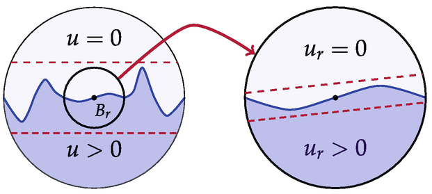
Improvement of flatness in the ball B 1. For simplicity, we set r := r 0
-
The flatness direction does not change (ν′ = ν). Notice that, without changing the direction, the improvement of flatness (in the sense of Theorem 7.4) should not hold. In fact, the function \(u(x)=x_d^+\) is ε-flat in the direction ν (whenever |ν − e d| = ε), but for any r > 0, \(u_r(x)=u(x)=x_d^+\), thus u r cannot be more than ε-flat in the direction ν (the improvement is only possible if we are allowed to replace ν by a vector, which is closer to e d).

The main result of this section is the following.
Theorem 7.7 (Partial Boundary Harnack)
There are dimensional constants \(\bar {\varepsilon }>0\) and c ∈ (0, 1) such that for every viscosity solution u of (7.2) in \(B_1\subset \mathbb {R}^d\) such that \(0\in \overline \Omega _u\) we have the following property:
If there are two real numbers a 0 < b 0 such that
then there are real numbers a 1 and b 1 such that a 0 ≤ a 1 < b 1 ≤ b 0,
Proof
Since \(0\in \overline \Omega _u\) we have that a 0 ≥−1∕10. We consider two cases:
-
1.
Suppose that |a 0|≤ 1∕10. Then applying Lemma 7.10 we have the claim.
-
2.
Suppose that a 0 ≥ 1∕10. Then u is harmonic in B 1 ∩{x d > −1∕10} (and so, in the ball B 1∕10) and the claim follows by Lemma 7.9.
□
We next prove the two main results: Lemmas 7.9 and 7.10. Section 7.2.1 is dedicated to the proof of Lemma 7.9, which is a consequence of the classical Harnack inequality for harmonic functions stated in Lemma 7.8. Section 7.2.2 is dedicated to the boundary version of the Harnack inequality (Lemma 7.10), which is due to De Silva [23].
7.2.1 Interior Harnack Inequality
Lemma 7.8 (Harnack Inequality)
There is a dimensional constant \(C_{\mathcal H}\) such that for every \(h:B_{2r}(x_0)\to \mathbb {R}\) , a non-negative harmonic function in the ball \(B_{2r}(x_0)\subset \mathbb {R}^d\) , the following (Harnack) inequality does hold
In particular, we have
Proof
The proof is an immediate consequence of the mean-value property. □
Lemma 7.9 (Improvement of Flatness at Fixed Scale)
Let \(C_{\mathcal H}>1\) be the dimensional constant from the Harnack inequality (7.4) and let \(c_{\mathcal H}:=\big (2C_{\mathcal H}\big )^{-1}\) . Suppose that \(u:B_{2r}\to \mathbb {R}\) is a harmonic function for which there are a constant ε > 0 and a linear function \(\ell :\mathbb {R}^d\to \mathbb {R}\) such that
Then at least one of the following does hold :
-
(i)
\(\ell (x)+c_{\mathcal H}{\varepsilon }\le u(x)\le \ell (x)+{\varepsilon }\quad \mathit{\text{for every}}\quad x\in B_{r}\);
-
(ii)
\(\ell (x)\le u(x)\le \ell (x)+(1-c_{\mathcal H}){\varepsilon }\quad \mathit{\text{for every}}\quad x\in B_{r}\).
Proof
We consider two cases.
Case 1. Suppose that u(0) ≥ ℓ(0) + ε∕2. Then the function h := u − ℓ is harmonic and non-negative in B 2r. Then, by the Harnack inequality (7.4), we have
which means that
and so (i) holds.
Case 2. Suppose that u(0) ≤ ℓ(0) + ε∕2. Then the function h := ℓ + ε − u is harmonic and non-negative in B 2r. Then, by the Harnack inequality (7.4), we have
which means that
and so (ii) holds. □
7.2.2 Partial Harnack Inequality at the Free Boundary
Lemma 7.10 (Improving the Flatness at Fixed Scale; De Silva [23])
There are dimensional constants \(\bar {\varepsilon }>0\) and c ∈ (0, 1), for which the following does hold.
Suppose that \(u:B_1\to \mathbb {R}\) is a continuous non-negative function and a viscosity solution of (7.2) in \(B_1\subset \mathbb {R}^d\) . Then, we have the following property:
If there are real constants ε and σ, \(0<{\varepsilon }\le \bar {\varepsilon }\) and |σ| < 1∕10, such that
then at least one of the following does hold :
-
(i)
(x d + σ + cε)+ ≤ u(x) ≤ (x d + σ + ε)+ for every x ∈ B 1∕20 ;
-
(ii)
(x d + σ)+ ≤ u(x) ≤ (x d + σ + (1 − c)ε)+ for every x ∈ B 1∕20.
Proof
We set
and consider the function \(w:\mathbb {R}^d\to \mathbb {R}\), defined as (see Fig. 7.2):


The function w
The set, where the function w is not constantly vanishing, is precisely the ball \(B_{{3}/{4}}(\bar x)\) (see Fig. 7.2). Moreover, on the annulus  , the function w has the following properties :
-
(w1)
\(\displaystyle \Delta w(x)=2\,d\,\bar c \,|x-\bar x|{ }^{-(d+2)}\ge 2\,d\,\bar c\, \big ({4}/{3}\big )^{d+2}>0\ \).
-
(w2)
\(\displaystyle \partial _{x_d}w\ge C_{w}>0\) on the half-space {x d < 1∕10}. Here, C w > 0 is an (explicit) constant depending only on the dimension.
Following the notation from [23] we set p(x) = x d + σ. Similarly to what we did in the proof of Lemma 7.9, we consider two cases.
Case 1. Suppose that \(u(\bar x)\ge p(\bar x)+\frac {{\varepsilon }}2\).
Since the function u − p is harmonic and non-negative in the ball \(B_{{1}/{10}}(\bar x)\), we can apply the Harnack inequality (7.4). Thus, setting \(c_{\mathcal H}:=\big (2C_{\mathcal H}\big )^{-1}\) we get
We now consider the family of functions
We will prove that for every t ∈ [0, 1), we have u(x) ≥ v t(x) in B 1. We notice that, for t < 1 the function v t has the following properties:
-
(v1)
v t(x) < p(x) ≤ u(x) on
 (since the support of w is precisely \(B_{{3}/{4}}(\bar x)\)),
 -
(v2)
v t(x) < u(x) in \(\overline B_{\frac 1{20}}(\bar x)\) (by the choice of the constant \(c_{\mathcal H}\)),
-
(v3)
Δv t(x) > 0 on the blue annulus
 (follows from (w1)),
 -
(v4)
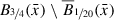
\(|\nabla v_t|(x)\ge \partial _{x_d}v_t(x)\ge 1+ c_{\mathcal H}{\varepsilon } C_w>1\) on
 .
.
 (since the support of w is precisely
  (follows from (w1)),
 .
. Suppose (by absurd) that, for some t ∈ [0, 1), the function u − v
t has local minimum in B
1 in a point \(x\in \overline B_1\). By (v3) and the fact that u is a viscosity solution we have that  . By (v4) we have that
  and
and  . Thus we get
  . By (v1) and (v2) we conclude that
Thus, we obtain that u ≥ v 1 on \(\overline B_1\), i.e.
Now since w is strictly positive on the ball B 1∕20 we get that
which proves that the property (i) holds.
Case 2. Suppose that \(u(\bar x)< p(\bar x)+\frac {{\varepsilon }}2\).
Since the function p + ε − u is harmonic and non-negative in the ball \(B_{{1}/{10}}(\bar x)\), we can apply the Harnack inequality, thus obtaining that for a dimensional constant \(c_{\mathcal H}>0\) we have
We now consider the family of functions
and, reasoning as in the previous case, we get that
In particular, since w is strictly positive on the ball B 1∕20, we get that
which concludes the proof. □
7.3 Convergence of Flat Solutions
In this subsection we prove the compactness result that we will need in the proof of Theorem 7.4. The proof is entirely based on Theorem 7.7, from which we know that any (continuous, non-negative) viscosity solution \(u:B_1\to \mathbb {R}\) of (7.2) satisfies the following condition.
Condition 7.11 (Partial Improvement of Flatness)
There are constants \(\bar {\varepsilon }>0\) and c ∈ (0, 1) such that the following holds. If \(x_0\in \overline \Omega _u\) , B r(x 0) ⊂ B 1 and a 0 < b 0 are such that
then there are real numbers a 1 and b 1 such that a 0 ≤ a 1 < b 1 ≤ b 0,
Remark 7.12
We notice that if \(u:B_1\to \mathbb {R}\) is a continuous non-negative function on B 1, then, for any a < b and any set E ⊂ B 1, the inequality
is equivalent to
Thus, an equivalent way to state Condition 7.11 is the following. The non-negative function \(u:B_1\to \mathbb {R}\) satisfies Condition 7.11, if and only if, the following holds.
If \(x_0\in \overline \Omega _u\), B r(x 0) ⊂ B 1 and a 0 < b 0 are such that
then there are real numbers a 1 and b 1 such that a 0 ≤ a 1 < b 1 ≤ b 0,
The constants \(\bar {\varepsilon }\) and c are the same as in Condition 7.11.
Lemma 7.13
Suppose that the continuous non-negative function \(u:B_1\to \mathbb {R}\) satisfies Condition 7.11 with constants c and \(\bar {\varepsilon }\) . Suppose that \(0\in \overline \Omega _u\) and that there are two real numbers a 0 < b 0 such that
Then, setting
for every \(x_0\in B_{{1}/{2}}\cap \overline \Omega _{u}\) , we have the uniform estimate

where C is a numerical constant and γ depends only on c.
Proof
Let n ≥ 0 be such that
Let \(\displaystyle r_j=\frac 12\big ({1}/{20}\big )^{j}.\) Then, we have
Thus, for every \(x_0\in B_{1/2}\cap \overline \Omega _u\) we can apply the (partial) improvement of flatness in \(B_{r_j}(x_0)\), for every j = 0, 1, …, n. Thus, we get that there are
such that
which implies that
and so,
The triangular inequality implies that
which gives the claim by choosing j such that
and setting γ to be such that (1∕20)γ = 1 − c. □
Lemma 7.14 (Compactness for Flat Sequences)
Let \(\bar {\varepsilon }>0\) and c ∈ (0, 1) be fixed constants. Suppose that \(u_k: B_1\to \mathbb {R}\) is a sequence of continuous non-negative functions such that
-
(a)
u k satisfies Condition 7.11 in B 1 with constants \(\bar {\varepsilon }\) and c.
-
(b)
u k is ε k -flat in B 1 , that is,
$$\displaystyle \begin{aligned} x_d-{\varepsilon}_k\le u_k(x)\le x_d+{\varepsilon}_k\quad \mathit{\text{in}}\quad B_1\cap\overline\Omega_{u_k}. \end{aligned}$$ -
(c)
limk→∞ ε k = 0.
Then there is a Hölder continuous function \(\widetilde u : B_{{1}/{2}}\cap \{x_d\ge 0\}\to \mathbb {R}\) and a subsequence of
that we still denote by \(\tilde u_k\) such that the following claims do hold.
-
(i)
For every δ > 0, \(\tilde u_k\) converges uniformly to \(\widetilde u\) on the set B 1∕2 ∩{x d ≥ δ}.
-
(ii)
The sequence of graphs
$$\displaystyle \begin{aligned} \Gamma_k=\big\{(x,\tilde u_k(x))\ :\ x\in \overline\Omega_{u_k}\cap B_{{1}/{2}}\big\}\subset \mathbb{R}^{d+1}, \end{aligned}$$converges in the Hausdorff distance (in \(\mathbb {R}^{d+1}\) ) to the graph
$$\displaystyle \begin{aligned} \Gamma=\big\{(x,\tilde u(x))\ :\ x\in B_{{1}/{2}}\cap \{x_d\ge 0\}\big\}. \end{aligned}$$
Proof
We first prove (i). For every \(y\in B_{{1}/{2}}\cap \overline \Omega _{u_k}\) we have that
Thus, by Lemma 7.13 we have that \(\tilde u_k\) satisfies
which, since y is arbitrary, gives
Since, for ε k ≤ δ, we have that \(\{x_d\ge \delta \}\cap B_{1}\subset \Omega _{u_k}\cap B_1\), we get that the sequence \(\tilde u_k : \{x_d\ge \delta \}\cap B_{{1}/{2}}\to \mathbb {R}\) satisfies :
-
\(\tilde u_k\) is equi-bounded on {x d ≥ δ}∩ B 1∕2
$$\displaystyle \begin{aligned} -1=\frac{(x_d-{\varepsilon}_k)-x_d}{{\varepsilon}_k}\le \frac{u_k(x)-x_d}{{\varepsilon}_k}\le\frac{(x_d+{\varepsilon}_k)-x_d}{{\varepsilon}_k}=1 ; \end{aligned}$$ -
\(\tilde u_k\) satisfies
$$\displaystyle \begin{aligned} \text{osc}\,\big(\tilde u_k ; {A_{2r,r}(x_0)\cap \{x_d\ge \delta\}\cap B_{{1}/{2}}}\big)\le 2Cr^\gamma\qquad \text{for every}\qquad r\ge \frac{{\varepsilon}_k}{\bar{\varepsilon}}, \end{aligned}$$where, for any set \(E\subset \overline \Omega _{u_k}\), we define:
$$\displaystyle \begin{aligned} \text{osc}\,(\tilde u_k ; E):=\sup_{E} \tilde u_k-\inf_{E}\tilde u_k, \end{aligned}$$and, for every 0 < r < R, A R,r(x 0) is the annulus


Thus, by the Ascoli-Arzelà Theorem, there is a subsequence converging uniformly on the set {x d ≥ δ}∩ B 1∕2 to a Holder continuous function
satisfying
The above argument does not depend on δ > 0. Thus, the function \(\tilde u\) can be defined on the entire half-ball {x d > 0}∩ B 1∕2. Moreover, the constants C and γ do not depend on the choice of δ > 0. This implies that we can extend \(\tilde u\) to a Hölder continuous function
still satisfying the uniform continuity estimate
We now prove (ii). Suppose that \(\tilde x=(x,\tilde u(x))\in \Gamma \). For every δ > 0, there is a point y ∈ B 1∕2 ∩{x d > δ∕2} such that |x − y|≤ δ. (Notice that, if x ∈ B 1∕2 ∩{x d > δ∕2}, then we can simply take y = x.) Then, setting \(\tilde y=(y,\tilde u(y))\), we have the estimate
On the other hand, for every k such that ε k ≤ δ, we have
Thus, we finally obtain the estimate
Let now \(\tilde x_k=\big (x_k,\tilde u_k(x_k)\big )\in \Gamma _k\). Let k be such that \({{\varepsilon }_k}/{\bar {\varepsilon }}\le \frac {\delta }2\). Let y k ∈{x d ≥ δ}∩ B 1∕2 be such that δ∕2 ≤|x k − y k|≤ 2δ and let \(\tilde y_k=\big (y_k,\tilde u_k(y_k)\big )\). Then, we have
Reasoning as above, we get
Now, since δ is arbitrary and \(\tilde u_k\) converges to \(\tilde u\) uniformly on {x d > δ∕2}∩ B 1∕2, we get that
□
7.4 Improvement of Flatness: Proof of Theorem 7.4
In this subsection, we prove Theorem 7.4. Since, we will reason by contradiction, we will first study the limits of the sequences of (flat) viscosity solutions to (7.2) in B 1.
Lemma 7.15 (The Linearized Problem)
Suppose that \(u_k:B_1\to \mathbb {R}\) is a sequence of continuous non-negative functions such that:
-
(a)
for every k, u k is a viscosity solution of
$$\displaystyle \begin{aligned} \Delta u_k=0\quad \mathit{\text{in}}\quad \Omega_{u_k}\cap B_1\ ,\qquad |\nabla u_k|=1\quad \mathit{\text{on}}\quad \partial \Omega_{u_k}\cap B_1. \end{aligned} $$(7.5) -
(b)
for every k, u k is ε k -flat in B 1 in the sense that
$$\displaystyle \begin{aligned} (x_d-{\varepsilon}_k)_+\le u_k(x)\le (x_d+{\varepsilon}_k)_+\qquad \mathit{\text{in}}\qquad B_1. \end{aligned}$$ -
(c)
limk→∞ ε k = 0.
Then, up to extracting a subsequence, the sequence of functions
converges (in the sense of Lemma 7.14 (i) and (ii)) to a Hölder continuous function
Moreover, we have that
-
(i)
\(\tilde u\) is a viscosity solution to
$$\displaystyle \begin{aligned} \Delta \tilde u=0\quad \mathit{\text{in}}\quad B_{{1}/{2}}\cap \{x_d>0\}\ ,\qquad \frac{\partial \tilde u}{\partial x_d}=0\quad \mathit{\text{on}}\quad B_{{1}/{2}}\cap \{x_d=0\}\ , \end{aligned} $$(7.6)in the sense that
-
\(\tilde u\) is harmonic in B 1∕2 ∩{x d > 0},
-
If P is a polynomial touching \(\tilde u\) from below (above) in a point x 0 ∈ B 1∕2 ∩{x d = 0}, then \(\displaystyle \frac {\partial P}{\partial x_d}(x_0)\le 0\) \(\ \left (\displaystyle \frac {\partial P}{\partial x_d} (x_0)\ge 0\right )\).
-
-
(ii)
\(\tilde u\in C^{\infty }\big (B_{{1}/{2}}\cap \{x_d\ge 0\}\big )\) and is a classical solution of (7.6).
Proof
The existence of the limit function \(\tilde u\) follows by Lemma 7.14.
We first prove (i). Suppose that P is a polynomial touching \(\tilde u\) strictly from below in a point x 0 ∈ B 1∕2 ∩{x d ≥ 0}. Then there exists a sequence of points \(x_k\in \overline \Omega _{u_k}\) such that P touches \(\tilde u_k\) from below in x k and x k → x 0 as k →∞. We consider two cases:
-
(1)
Suppose that x 0 ∈{x d > 0}. Then there is some δ > 0 such that x k ∈{x d > δ}, for every k large enough. Thus, \(x_k\in \Omega _{u_k}\) for k large enough and so, since \(\tilde u_k\) is harmonic in \(\Omega _{u_k}\), ΔP(x k) ≥ 0. Passing to the limit as k →∞ we get ΔP(x 0) ≥ 0.
-
(2)
Suppose that x 0 ∈{x d = 0}. We suppose without loss of generality that x 0 = 0. We consider the family of polynomials
$$\displaystyle \begin{aligned} P_{{\varepsilon}} (x)=P(x)+ \frac 1{\varepsilon} x_d^2-{\varepsilon} x_d. \end{aligned}$$In a sufficiently small neighborhood of zero, we have that P ε still touches \(\tilde u\) (strictly) from below in 0. Moreover,
$$\displaystyle \begin{aligned} \Delta P_{\varepsilon}>0\quad \text{in a neighborhood of zero}\,,\qquad \frac{\partial P_{\varepsilon}}{\partial x_d}(0)=\frac{\partial P}{\partial x_d}(0)-{\varepsilon}. \end{aligned}$$Thus it is sufficient to show that for every ε > 0, we have \(\displaystyle \frac {\partial P_{\varepsilon }}{\partial x_d}(0)\le 0\). Let now ε > 0 be fixed. Consider the sequence of points \(x_k\in \overline \Omega _{u_k}\) such that P ε touches \(\tilde u_k\) from below in x k and x k → x 0 as k →∞. Since ΔP ε(x k) > 0 and \(\tilde u_k\) is harmonic in \(\Omega _{u_k}\) we have that necessarily x k ∈ ∂ Ωk. By the definition of \(\tilde u_k=\frac {u_k-x_d}{{\varepsilon }_k}\) we get that the polynomial Q(x) = ε k P ε(x) + x d touches u k from below in x k. Since u k is a viscosity solution of (7.5), we get that
$$\displaystyle \begin{aligned} 1\ge |\nabla Q(x_k)|{}^2\ge \Big(1+{\varepsilon}_k\frac{\partial P_{\varepsilon}}{\partial x_d}(x_k)\Big)^2= 1+2{\varepsilon}_k\frac{\partial P_{\varepsilon}}{\partial x_d}(x_k)+{\varepsilon}_k^2\left|\frac{\partial P_{\varepsilon}}{\partial x_d}(x_k)\right|{}^2. \end{aligned}$$Thus, we have \(\displaystyle \frac {\partial P_{\varepsilon }}{\partial x_d}(0)\le 0\), which concludes the proof after letting ε → 1.
We now prove (ii). We write \(\mathbb {R}^d\ni x=(x',x_d)\) with \(x'\in \mathbb {R}^{d-1}\) and \(x_d\in \mathbb {R}\). We consider the function \(w:\mathbb {R}^d\to \mathbb {R}\) defined by \(\tilde u\) and its reflexion:
We will prove that w is harmonic on \(\mathbb {R}^d\). Suppose that P is a polynomial touching w strictly from below in a point x 0 ∈{x d = 0}. Since w is harmonic on {x d ≠ 0} it is sufficient to prove that ΔP(x 0) ≤ 0. We first notice that since w(x′, x d) = w(x′, −x d) then also the polynomial P(x′, −x d) touches w strictly from below in x 0 and, as a consequence, so does the polynomial
which satisfies
Consider the polynomial
Then Q ε touches w from below in a point x ε and we have that x ε → x 0 as ε → 0. We notice that necessarily x ε ∈{x d ≥ 0}. Moreover, we can rule out the case x ε ∈{x d = 0} since by the hypothesis on \(\tilde u\) we have that in this case we should have
which is impossible. Thus x ε ∈{x d > 0} and since \(\tilde u\) is harmonic in {x d > 0} we get that
Passing to the limit as ε → 0, we obtain that ΔQ(x 0) ≤ 0, which concludes the proof. □
Lemma 7.16 (First and Second Order Estimates for Harmonic Functions)
Suppose that \(h:B_R\to \mathbb {R}\) is a bounded harmonic function in B R . Then
and
where C d is a dimensional constant.
Proof
Let x 0 ∈ B 3R∕4. Since h is harmonic in B R∕4(x 0), we have that also ∂ i h is harmonic in the same ball B R∕4(x 0), we have
where X = (0, …, h, …, 0) is the vector with the only non-zero component being the ith one, which is precisely h. Now, the divergence theorem gives
which implies that
and so, we obtain (7.7). Now, by the same argument, we get that
Let now x ∈ B R∕4 and set
Then, we have
Since
and
we get precisely (7.8). □
Proof of Theorem 7.4
We fix C 0 and r 0 to be dimensional constant which will be chosen later. In order to prove that ε 0 exists we reason by contradiction. Let ε n → 0 and let \(u_n:B_1\to \mathbb {R}\) be a sequence of continuous functions satisfying the conditions (a), (b) and (c) with ε n. Without loss of generality, we may suppose that, for any \(n\in \mathbb {N}\), u n is ε n flat in B 1 in the same direction e d. Finally, we assume by contradiction that, there are no \(n\in \mathbb {N}\) and a unit vector ν satisfying the following conditions:
(i) |ν − e d|≤ C 0 ε;
(ii) the function \((u_n)_{r_0}:B_1\to \mathbb {R}\) is σε-flat in B 1, in the direction ν.
By Lemma 7.14 we can suppose that the sequence
converges (in the sense of Lemma 7.14 (i) and (ii)) in B 1∕2 to a smooth (C ∞(B 1∕2)) function
that satisfies (7.6). We notice that
We set
and we re-write (7.8) as
We now fix r ≤ 1∕4. Since the graph Γn of \(\tilde u_n\) converges in the Hausdorff distance to the graph Γ of \(\tilde u\) (see Lemma 7.14 (ii)), we have that for n large enough
Using the definition of \(\tilde u_n\) we can rewrite (7.9) as
which holds for every \(x=(x',x_d)\in B_r\cap \overline \Omega _{u_n}\).
We define the new flatness direction ν as follows:
By definition, we have that |ν| = 1. We next estimate the distance between ν and e d. Since both ν and e d are unit vectors, we have
Notice that the following elementary inequality holds:
In order to apply this inequality to \(X={\varepsilon }_n^2|\nu '|{ }^2\), we first check that \({\varepsilon }_n^2|\nu '|{ }^2\le {1}/{2}\). In fact, by the definition of ν′ and (7.7), we have the estimate |ν′|≤ 2C d. Thus, for n large enough, we have that \({\varepsilon }_n^2|\nu '|{ }^2\le {1}/{2}\) and so, we can estimate
which proves that ν satisfies (i), once we choose C 0 = 4C d.
Using again the inequality (7.11) and the fact that
which follows by the non-negativity and the ε n-flatness of u n, we get that
Thus, dividing (7.10) by \(\sqrt {1+{\varepsilon }_n^2|\nu '|{ }^2}\), we get that
for every \(x=(x',x_d)\in B_r\cap \overline \Omega _{u_n}\), C d being a dimensional constant. Choosing r 0 small enough and ε 0 ≤ r 0, we get that
and so the vector ν satisfies (i) and (ii), in contradiction with the initial assumption. □
References
D. De Silva, Free boundary regularity for a problem with right hand side. Interfaces Free Bound. 13 (2), 223–238 (2011)
Author information
Authors and Affiliations
Rights and permissions
Open Access This chapter is licensed under the terms of the Creative Commons Attribution 4.0 International License (http://creativecommons.org/licenses/by/4.0/), which permits use, sharing, adaptation, distribution and reproduction in any medium or format, as long as you give appropriate credit to the original author(s) and the source, provide a link to the Creative Commons license and indicate if changes were made.
The images or other third party material in this chapter are included in the chapter's Creative Commons license, unless indicated otherwise in a credit line to the material. If material is not included in the chapter's Creative Commons license and your intended use is not permitted by statutory regulation or exceeds the permitted use, you will need to obtain permission directly from the copyright holder.
Copyright information
© 2023 The Author(s)
About this chapter

Cite this chapter
Velichkov, B. (2023). Improvement of Flatness. In: Regularity of the One-phase Free Boundaries. Lecture Notes of the Unione Matematica Italiana, vol 28. Springer, Cham. https://doi.org/10.1007/978-3-031-13238-4_7
Download citation
DOI: https://doi.org/10.1007/978-3-031-13238-4_7
Published:
Publisher Name: Springer, Cham
Print ISBN: 978-3-031-13237-7
Online ISBN: 978-3-031-13238-4
eBook Packages: Mathematics and StatisticsMathematics and Statistics (R0)