
Abstract
In this chapter we discuss how the intensional account of harmony sketched in the first chapter can be developed in a systematic way for a class of connectives whose rules are obtained in a uniform way using an inversion principle. To handle disjunction and disjunction-like connectives, the formulation of the expansions requires particular care. We discuss and compare two different ways of formulating the inversion principle and finally we investigate the prospects of developing an account of harmony for connectives whose rules do not obey inversion, pointing at the weakness of the approaches proposed in the literature so far.
You have full access to this open access chapter, Download chapter PDF
1 Disjunction: A Problem for Stability
The account of harmony in terms of reductions and expansions sketched in Sect. 1.3 encounters a difficulty when one tries to apply it to the rules of disjunction:

As in the case of conjunction, it is quite uncontroversial that the rules satisfy both aspects of the informal characterization of harmony, and in fact deductive patterns of the two kinds discussed, as well as reductions and expansions can be exhibited in this case as well:


Besides these rules for disjunction (which in most formulations are common to both intuitionistic and classical logic), Dummett [12] discusses also those for quantum disjunction (more commonly referred to as lattice disjunction) \(\mathbin {\overline{\vee }}\). The rules for this connective differ from those of standard disjunction in that the elimination rule comes with a restriction, to the effect that the rule can be applied only when the minor premises C depend on no other assumptions apart from those that get discharged by the rule application (we indicate this using double square brackets in place of the usual ones):

Using the elimination rule for quantum disjunction one can derive from \(A\mathbin {\overline{\vee }} B\) less than what one can derive from \(A\vee B\) using \(\vee \)E . Thus, on the assumption that the standard rules for disjunction are in perfect balance, we expect the rules for quantum disjunction not to be in perfect harmony.1 In particular, we expect the no less aspect of harmony not to be met.2 That is, we expect the rules for \(\mathbin {\overline{\vee }}\) to be unstable.3
However, and here is the problem, reductions and expansions are readily available in the case of quantum disjunction as well (again with double square brackets we indicate that no other assumption (apart from those indicated) occurs in \(\mathscr {D}_1\) and \(\mathscr {D}_2\)):

Observe in particular that the restriction on \(\mathbin {\overline{\vee }}\)E is satisfied by the applications of the rule in the expanded derivations and thus that, though unstable, the restricted elimination rule allows one to derive from \(A\mathbin {\overline{\vee }}B\) no less than what is needed in order introduce \(A\mathbin {\overline{\vee }}B\) back again.
Most authors (see, e.g. [4, 103]) have taken the modest stance of regarding instabilities of this kind as too subtle to be ruled out by the existence of expansions. Here we will argue against this modest stance, by showing that, once properly formulated, expansions are perfectly capable of detecting instabilities of this kind.
2 A “Quantum-Like” Implication
Before reformulating the expansion pattern for disjunction, we would like to point at some independent evidence in favor of the view that the existence of expansions should rule out instabilities of this kind. In so doing, we hope to dispel the possibly mistaken impression that our solution to the problem of quantum disjunction is merely ad hoc.
Evidence in favor of our bolder stance towards stability and expansions arises when one considers a restriction on \(\mathbin {\supset }\)I analogous to the one yielding quantum disjunction also briefly discussed by Dummett [12, p. 289] as a case of instability. Let \(\mathbin {\overline{\mathbin {\supset }}}\) be the “quantum-like” implication connective governed by the following rules:

where the introduction rule is restricted to the effect that it can be applied only when the premise B depends on no other assumptions apart from those that get discharged by the rule application.
The restricted introduction rule sets higher standards for inferring a proposition of the form \(A\mathbin {\overline{\mathbin {\supset }}} B\) than those set by \(\supset \)I to derive a proposition of the form \(A\mathbin {\supset }B\). Thus, on the assumption that \(\mathbin {\supset }\)E is in perfect harmony with the standard introduction rule, we expect \(\mathbin {\overline{\mathbin {\supset }}}\)E not to be in perfect harmony with the restricted introduction rule. In particular, as the restricted introduction rule sets higher standards to derive an implication, we expect that using \(\mathbin {\overline{\mathbin {\supset }}}\)E we cannot derive from \(A\mathbin {\overline{\mathbin {\supset }}} B\) all that is needed to introduce \(A\mathbin {\overline{\mathbin {\supset }}} B\) again using its introduction rule. In other words, we expect also in this case the no less aspect of harmony not to be met. That is we expect the rules for \(\mathbin {\overline{\mathbin {\supset }}}\) to be unstable, the kind of instability at stake being the same as the one flawing the rules for \(\mathbin {\overline{\vee }}\).4
As in the case of \(\mathbin {\overline{\vee }}\), in the case of \(\mathbin {\overline{\mathbin {\supset }}}\) we have a reduction readily available which shows that—as expected—the no more aspect of harmony is satisfied:

Moreover, it is easy to see that the expansion pattern for standard implication does not work for quantum-like implication, as the application of \(\mathbin {\overline{\mathbin {\supset }}}\)I would violate the restriction that the premise B depends on no other assumptions than the one that get discharged by the rule: In the expanded pattern B would depend not only on A but also on all assumptions on which \(A\mathbin {\overline{\mathbin {\supset }}}B\) depends:

The requirement that it should be possible to equip the rules with both reductions and expansions is thus capable of detecting the instability of the rules of quantum-like implication. We take this as a reason to consider an alternative pattern for the expansion of disjunction, namely one capable of detecting the disharmony induced by the restriction on the quantum disjunction elimination rule.5
3 Generalizing the Expansions for Disjunction
The expansion pattern for disjunction (\(\vee \eta \)) we considered above—which was first proposed by Prawitz [66]—gives the instructions to expand a derivation in which the disjunctive proposition figures as conclusion of the whole derivation.
The idea behind the alternative pattern is that an expansion operates on a formula which is not, in general, the conclusion of a derivation, but on one that occurs at some point in the course of a derivation. Consider a derivation \(\mathscr {D}\) in which the formula \(A\vee B\) may occur at some point. Such a derivation may be depicted as follows:

—that is, it may be viewed as the result of plugging a (certain number \(k\ge 0\)) of copies of a derivation \(\mathscr {D}'\) of \(A\vee B\) on top of a derivation \(\mathscr {D}''\) of C depending on (k copies of) the assumption \(A\vee B\), possibly alongside other assumptions \(\Gamma \).
It is certainly true that Prawitz’s expansion (\(\vee \eta \)) can also be used to expand a derivation \(\mathscr {D}\) of this form: To expand \(\mathscr {D}\), we can apply Prawitz’s expansion to the upper chunk \(\mathscr {D}'\) of \(\mathscr {D}\) (in which \(A\vee B\) figures as conclusion), and then we can plug the result of the expansion on top of the lower chunk \(\mathscr {D}''\) of \(\mathscr {D}\), thereby obtaining the following:

It is however possible to define an alternative procedure to directly expand the whole of \(\mathscr {D}\), namely the following:

In the alternatively expanded derivation, the application of the elimination rule \(\vee \)E is postponed to the effect that its minor premises are not the two copies of \(A\vee B\) obtained respectively by \(\vee \)I\(_1\) and \(\vee \)I\(_2\) (as in Prawitz’s expansion), but rather two copies of C which are the conclusions of two copies of the lower chuck \(\mathscr {D}''\) of \(\mathscr {D}\) that now constitute the main part of the derivations of the minor premises of the application of \(\vee \)E.
This alternative pattern, first proposed by Seely [97], is a generalization of Prawitz’s expansion pattern: Each instance of Prawitz’s pattern (\(\vee \eta \)) corresponds to an instance of the alternative pattern (\(\vee \eta _g\)) in which the lower chunk \(\mathscr {D}''\) of the derivation \(\mathscr {D}\) is “empty” i.e. it just consists of the proposition \(A\vee B\).
Moreover, it is easy to see that we cannot replace \(\vee \) with \(\mathbin {\overline{\vee }}\) in the above pattern for generalized expansions, since the application of \(\mathbin {\overline{\vee }}\)E in the expanded derivation would violate the quantum restriction: The minor premises C would not depend only on the assumptions of the form A and B that get discharged by the rules, but also on all other undischarged assumptions of \(\mathscr {D}''\):

Thus, quantum disjunction does turn out to be unstable (in accordance with what we would expect), provided that stability is understood as the existence of generalized expansions.
What the alternative expansion expresses is a generalization of the no less aspect of harmony that could be roughly approximated as follows:
The elimination rule allows one to derive no less than what is needed to derive all consequences from a logically complex proposition of a given form.
Starting from the alternative formulation of harmony given by Negri and von Plato [53]: “whatever follows from the direct grounds for a proposition must follow from that proposition.” (see also Note 5 to Chap. 1 above) one may propose the following as the proper way of understanding harmony:
Harmony: Informal statement 1
What can be inferred from the direct grounds for a proposition A together with further propositions \(\Gamma \) should be no more and no less that what follows from A together with \(\Gamma \).
4 Harmony: Arbitrary Connectives and Quantifiers
Prawitz [69] first proposed a general procedure to map any arbitrary collection of introduction rules onto a specific collection of elimination rules which is in harmony with the given collection of introduction rules. We will refer to such procedures as inversion principles.6 Prawitz’s procedure has been refined by Schroeder-Heister [85, 86, 94] in a deductive framework that generalizes the key ingredients of standard natural deduction calculi called the calculus of higher-level rules. We will therefore refer to the Prawitz–Schroeder-Heister procedure to generate elimination rules from a given collection of introduction rules as \(\texttt{PSH}\)-inversion.
The details of the calculus of higher-level rules and a more general presentation of PSH-inversion for rules of propositional connectives will be given in the Appendix A (see in particular Sect. A.9). In the present section, we informally give these results for the simplest case which does not require rules of higher level, and we suggest how \(\texttt{PSH}\)-inversion could be generalized to cover rules for arbitrary first-order quantifiers as well.
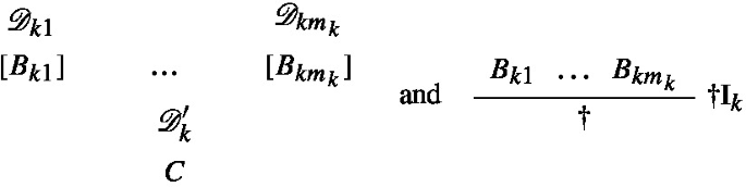
In this chapter we will assume \(\dagger \) to be an n-ary connective, and \(\dagger \textbf{I}\) to be a collection of \(r\ge 0\) distinct introduction rules for \(\dagger \) of the following form:

satisfying the following condition: for all \(1\le k\le r\), either \(m_k=0\) or for all \(1 \le j \le m_k\) there is an \(1\le i\le n\) such that \(B_{kj}\) is syntactically identical to \(A_i\). (Introduction rules of a more general kind are discussed in Appendix A, see in particular Sect. A.9.)
Definition 3.1
(\(\texttt{PSH}\)-inversion) Let \(\dagger \) and \(\dagger \textbf{I}\) be as above. We indicate with \(\texttt{PSH}(\dagger \textbf{I})\) the collection of elimination rules containing only the following rule:

where C is distinct from each \(A_i\).
We say that \(\dagger \) is a PSH-connectives in a calculus \(\texttt{K}\) iff \(\texttt{K}\) includes \(\dagger \textbf{I}\) and \(\texttt{PSH}(\dagger \textbf{I})\), and \(\dagger \) does not occur in any other of the primitive rules of \(\texttt{K}\).7
Let \(\texttt{K}\) be a calculus in which \(\dagger \) is a \(\texttt{PSH}\)-connective. In every \(\texttt{K}\)-derivation, one can get rid of any maximal formula occurrence governed by \(\dagger \) as follows (we abbreviate \(\dagger (A_1,\ldots ,A_n)\) with \(\dagger \)):

Moreover, given a \(\texttt{K}\)-derivation \(\mathscr {D}'\) of C depending on some assumptions of the form \(\dagger (A_1,\ldots ,A_n)\) and a \(\texttt{K}\)-derivation \(\mathscr {D}\) of \(\dagger (A_1,\ldots ,A_n)\) we can define the following generalized \(\eta \)-expansion (again we abbreviate \(\dagger (A_1,\ldots ,A_n)\) with \(\dagger \); freshness conditions on the discharge indeces will be left implicit henceforth):

The disjunction rules of \(\texttt{NI}\) are obtained by instantiating these schemata for \(r=2\) and \(m_1=m_2=1\). To give a further example, for \(r=1\) and \(m_1=2\) we obtain the well-known variant of the rules for conjunction in which the two elimination rules of \(\texttt{NI}\) are replaced by the so-called general elimination rule for conjunction8:

for which we have the following reduction and (generalized) expansion:

We intend the schema to cover also the limit case of \(m=0\) that gives us the standard intuitionistic rules for \(\bot \):

for which we have no reduction but the following (generalized) expansion:

As we detail in the Appendix, in the setting of Schroeder-Heister’s calculus of higher-level rules the above schemata cover also the cases in which the \(B_{kj}\)s are not formulas (i.e. rules of lowest level), but rules of arbitrary (finite) level.9 For example, take \(\mathord {\supset }\textbf{I}\) to be the collection of introduction rules consisting only of the standard introduction rules for implication \(\supset \)I:

The collection of elimination rules \(\texttt{PSH}(\mathord {\supset }\textbf{I})\) consists of the following rule:

Using the notation that is introduced in the appendix, the reduction associated with these rules can be depicted as follows:

To give the reader at least an informal clarification of the notation involved in the reduction, we observe the following. A derivation of the rule \(A\Rightarrow B\) is equated by definition with a derivation of B from A, thus the derivation \(\mathscr {D}\) of B from A is ipso facto a derivation of \(A\Rightarrow B\). The result of substituting the derivation \(\mathscr {D}\) of \(A\Rightarrow B\) for the rule assumption \(A\Rightarrow B\) in \(\mathscr {D}'\) can be informally described as the derivation which results by removing all applications of the assumption rule \(A\Rightarrow B\) in \(\mathscr {D}'\) and inserting \(\mathscr {D}\) to fill the gap, i.e. by successively replacing all patterns of the form on the right with patterns of the form on the left.

Observe that depending on the number of copies of the assumption A in \(\mathscr {D}\) and the number of applications of \(A\Rightarrow B\) in \(\mathscr {D}'\), the operation requires a quite involved transformation already for a rule of almost lowest level such as \(A\Rightarrow B\). For exact definitions (covering rules of arbitrary level) see Appendix A.
The (generalized) expansion is the following:

It should be clear that the schemata above can be generalized to apply to more general collections of introduction rules which may not only be of arbitrary high level but which may also contain propositional quantification as in Schroeder-Heister [94]. A generalization covering also first-order quantification is possible too and expectedly straightforward. We limit ourselves to discuss a (hopefully suggestive) example, the rules characterizing a binary quantifier encoding the I corner of the traditional square of oppositions (“Some A are B”). The collections of introduction and elimination rules \(I\textbf{I}\) and \(\texttt{PSH}(I\textbf{I})\) consist of the following two rules respectively:

Also for these collections of rules we have a reduction and a (generalized) expansion following the pattern of those of the rules of conjunction with the elimination rule in general form:

5 Stability and Permutations
When calculi containing connectives with rules obeying \(\texttt{PSH}\)-inversion are considered, such as the full calculus \(\texttt{NI}\), one usually considers further conversions besides reductions and expansions. A typical example of further conversions are permutative conversions. The result of applying such conversions is a change in the order of application of certain rules within derivations. Permutative conversions were first introduced by Prawitz [65, Chap. IV] with the goal of extending the subformula property of \(\beta \)-normal derivations to the whole of \(\texttt{NI}\). Although \(\beta \)-normal (and \(\beta _w\)-normal) derivations in \(\texttt{NI}\) are canonical (i.e. Fact 3 holds for \(\texttt{NI}\)), \(\beta \)-normal derivations might contain occurrences of formulas which are neither a subformula of the undischarged assumptions nor of the conclusion. The following derivation in \(\texttt{NI}\) displays this fact (the example is taken from [26]):

The failure of the subformula property is triggered by the fact that, due to its peculiar form, the application of \(\vee \)E “hides” the fact that the formula \(A\wedge A\) is introduced (in both derivations of the minor premises of the application of \(\vee \)E) and then eliminated.
Prawitz [65] characterized the “hidden” redundancies of this kind in \(\texttt{NI}\) as maximal segments. Segments are defined as follows:
Definition 3.2
A segment (of length n) in a derivation is a sequence of formula occurrences \(A_1, \ldots , A_n\) of the same formula A such that
-
1.
for \(n>1\), for all \(i<n\) \(A_i\) is a minor premise of an application of \(\vee \)E with conclusion \(A_{i+1}\).
-
2.
\(A_n\) is not the minor premise of an application of \(\vee \)E;
-
3.
\(A_1\) is not the consequence of an application of \(\vee \)E.
Note that in the above derivation the only two segments of length 2 are those consisting (respectively) of one of the two minor premises followed by the consequence of the application of \(\vee \)E. All other formula occurrences in the derivations constitute segments of length 1.
Definition 3.3
A segment \(A_1,\ldots A_n\) is maximal iff \(A_1\) is the consequence of an application of an introduction rule or of \(\bot \)E and \(A_n\) is the major premise of an application of an elimination rule.10
In the above derivation both segments of lengths 2 are maximal. Note that maximal formula occurrences in \(\texttt{NI}^{\wedge \mathbin {\supset }}\) are a limit case of maximal segments (i.e. maximal segments of length 1).
Whereas applications of \(\beta \)-reductions allow one to get rid of maximal formula occurrences (i.e. maximal segments of length 1), permutative conversions can be used to shorten the length of maximal segments. The permutative conversions for disjunction (which we will indicate as \(\vee \gamma \)) can be schematically depicted as follows (in the derivation schemata, \(\langle \mathscr {D}\rangle \) indicates the possible presence of minor premises in \(\dagger \)E, where \(\dagger \)E stands for the elimination rule of some connective \(\dagger \))11:

An application of (\(\vee \gamma \)) to the above derivation yields the following one:

which by two applications of \(\wedge \beta _1\) reduces to

Counterexamples to the subformula property in \(\texttt{NI}\) are triggered by applications of \(\bot \)E as well, as shown by the following derivation:

which contains an occurrence of a formula—viz. \(A\mathbin {\supset }B\)—which is not a subformula of either the undischarged assumptions or the conclusion. This formula occurrence constitutes a segment which qualifies as maximal according to Definition 3.3. Using the following permutative conversions for \(\bot \) one can get rid of such segments12:

In \(\texttt{NI}\), \(\beta \gamma \)-reduction is not only weakly normalizing, but also confluent and strongly normalizing. Moreover, by generalizing the notion of track used for \(\texttt{NI}^{\wedge \mathbin {\supset }}\) (see Sect. 1.5 above), it is possible to establish a result analogous to Fact 1, from which a result analogous to Fact 2 follows immediately, i.e. the subformula property for \(\beta \gamma \)-normal derivations in the full calculus \(\texttt{NI}\).13
For future reference we observe that if one restricts oneself to the calculus for the \(\{\mathbin {\supset },\bot \}\)-language fragment, to which we will refer as \(\texttt{NI}^{\mathbin {\supset }\bot }\), there is no need to modify the notion of track used for \(\texttt{NI}^{\wedge \mathbin {\supset }}\) and the subformula property for \(\beta \gamma \)-normal derivations follows from the following:
Fact 4
(The form of tracks) Each track \(A_1\ldots A_{i-1}, A_i, A_{i+1},\ldots A_n\) in a \(\beta \gamma \)-normal derivation in \(\texttt{NI}^{\mathbin {\supset }\bot }\) contains a minimal formula \(A_i\) such that
-
If \(i>1\) then \(A_j\) (for all \(1< j< i\)) is the premise of an application of an elimination rule of which \(A_{j+1}\) is the consequence and thereby \(A_{j+1}\) is a subformula of \(A_j\).
-
If \(n>i\) then \(A_i\) is the premise of either an application of \(\bot \)E or of an introduction rule.
-
If \(n>i\) then \(A_j\) (for all \(i< j< n\)) is the premise of an application of an introduction rule of which \(A_{j+1}\) is the consequence and thereby \(A_j\) is a subformula of \(A_{j+1}\).
Proof
For a derivation to be \(\beta \gamma \)-normal, in each track all applications of elimination rules must precede all applications of introduction rules, and if \(\bot \)E is applied in the track, its consequence is either the last element of the track or the premise of an introduction rule. This warrants the existence of a minimal formula in each track. Since a track ends whenever it “encounters” the minor premise of an application of \(\supset \)E, the subformula relationships between the members of a track hold (as it can be easily verified by checking the shape of the rules of \(\texttt{NI}^{\mathbin {\supset }\bot }\)). \(\square \)
It is worth observing that permutative conversions can be “simulated” using generalized \(\eta \)-expansions and \(\beta \)-reductions. In particular, in the case of (\(\vee \gamma \)) one can obtain the derivation on the right-hand side from the one on the left-hand side as follows. First apply a generalized expansion to the derivation on the left-hand side of (\(\vee \gamma \)) by instantiating in the schema for the generalized expansion (\(\vee \eta _g\)) \(\mathscr {D}'\) with \(\mathscr {D}_1\) and \(\mathscr {D}''\) with

thereby obtaining the following derivation:

in which the two rightmost occurrences of \(A\vee B\) constitute two local peaks. Their reduction yields the derivation on the right-hand side of \((\gamma \vee )\). (In the case of \(\bot \) the permutation is just an instance of the generalized \(\eta \)-expansion; for other connectives, see Sect. 3.7 below.)
The relevance of permutations to harmony and in particular to stability was already pointed out by Dummett [12] and has been recently stressed by Francez [17]. The fact that permutative conversions can be recovered from generalized expansions thus provides on the one hand further evidence for the significance of permutative conversions for an inferential account of meaning, and on the other hand it offers further reasons to view generalized expansions as the proper way to capture stability.
Actually, using the alternative expansion pattern one can recover a more general form of permutation, which we indicate as \(\vee \gamma _g\)-conversion, in which any chunk of derivation (and not only applications of elimination rule) can be permuted-up across an application of disjunction elimination [97]:

Conversely, this general form of permutation coupled with Prawitz’s simple form of expansion is as strong as the alternative form of expansion. More precisely, the equivalence relation induced by \(\beta \)-reductions, and generalized \(\eta _g\)-expansions is equivalent to the one induced by \(\beta \)-reductions, Prawitz’s \(\eta \)-expansions and the generalized permutative \(\gamma _g\)-conversions ([97], for a proof see [40]).
As it has been recently established [83], \(\beta \eta _g\)-equivalence (or equivalently \(\beta \eta \gamma _g\)-equivalence) is the maximum non-trivial notion of equivalence in the full language of \(\texttt{NI}\). The notion of \(\beta \eta _g\)-isomorphism (see Sect. 2.5) has been shown to decidable, but only in the absence of \(\bot \), whereas it is still an open question whether \(\beta \eta _g\)-isomorphism is decidable in the full language of \(\texttt{NI}\), though it is known that it is not finitely axiomatizable [33].
In contrast to \(\beta \gamma \)-reduction, \(\beta \gamma _g\) reduction is neither strongly normalizing nor confluent [1, 21, 40]. Due to the lack of confluence, it is thus difficult to make sense of the idea that \(\beta \gamma _g\)-normal derivations in \(\texttt{NI}\) represent proofs in the most direct way possible. The same proof may be represented by more than one \(\beta \gamma _g\)-normal derivation. Hence, without further ado there is no criterion of selecting one among the normal derivations belonging to the same equivalence class as “the” most direct way of representing a given proof.14 It therefore seems that in the case of the full language of \(\texttt{NI}\) it is hard to reconcile, on the one hand, the idea that maximality is the criterion to select the “correct” way of analyzing identity of proofs and, on the other hand, that conversions are means to transform a less direct representation of a proof into a more direct one. For these reasons, Girard famously referred to permutative conversions in \(\texttt{NI}\) as the ‘defects of the system’ (see [26], Sect. 10.1).
We conclude this section by observing that some authors (notably [63, 110]) argued in favour of calculi in which all elimination rules follow the pattern of disjunction elimination (Tennant refers to rules of this form as ‘parallelized elimination rules’, while von Plato as ‘general elimination rules’). However, to avoid the complications of rules of higher level, the following equivalent15 rule is adopted instead of the \(\texttt{PSH}\)-elimination rule for \(\mathbin {\supset }\):

The resulting natural deduction calculus, to which we will refer as \(\texttt{NI}\) \(_g\), bears a close correspondence to sequent calculus (in fact, a much closer correspondence than the original \(\texttt{NI}\)) and as such is particularly suited for automated proof search (see, e.g., [113], Sects. 2.3.4 and 2.3.7).
For reasons analogous to those discussed in connection with the rule of disjunction elimination in \(\texttt{NI}\), in \(\texttt{NI}\) \(_g\) permutative conversions are associated to all elimination rules. As in the case of disjunction, one can distinguish between permutative conversions involving only elimination rules (analogous to \(\vee \gamma \) above) and permutative conversions of a more general form (analogous to \(\vee \gamma _g\)).
As in the case of \(\texttt{NI}\), \(\beta \gamma \)-reduction in \(\texttt{NI}\) \(_g\) is strongly normalizing and confuent (see [37] for a proof of strong normalization for the disjunction-implication fragment and [36] for a proof of confluence for the implication fragment alone; Matthes [46] claims that the proofs carry over to the full calculus), and the \(\beta \gamma \)-normal derivations can be concisely described as those derivations in which all major premises of elimination rules are in assumption position (or, in Tennant’s terminology ‘stand proud’). Neither strong normalization nor confluence however hold for the more general kind of permutative conversions.
Observe finally, that the adoption of elimination rules in general form jeopardizes the idea that normal derivations are the most direct way of denoting proofs already in the purely conjunctive fragment. For example, the following \(\texttt{NI}^{\wedge \mathbin {\supset }}\) \(\beta \)-normal derivation:

corresponds to the following two distinct \(\beta \gamma \)-normal derivations in the calculus in which \(\wedge \)E\(_{\texttt{PSH}}\) replaces \(\wedge \)E\(_1\) and \(\wedge \)E\(_2\):

Although they are both \(\beta \gamma \)-normal (and hence they are not \(\beta \gamma \)-equivalent), these two derivations are \(\gamma _g\)-equivalent: each can be obtained from the other by exchanging the order of the last two applications of \(\wedge \)E\(_\texttt{PSH}\).
The two derivations are two different representations of the same (function from) proof(s of the undischarged assumptions to proofs of the conclusion). However, neither of the two derivations can be said to represent their common denotation more directly than the other one.
In this sense (although maybe not in other respects), the natural deduction calculus \(\texttt{NI}^{\wedge \mathbin {\supset }}\) can be deemed superiour to the conjunction-implication fragment of \(\texttt{NI}\) \(_g\): the syntax of \(\texttt{NI}^{\wedge \mathbin {\supset }}\) “filters out” inessential differences such as the order in which inference rules are applied within derivations by enabling a more canonical representation of proofs.16
6 The Meaning of Harmony
As argued in Sect. 2.3, collections of introduction rules play the role of definitions. This can be understood as meaning not only that each introduction rule for \(\dagger \) expresses a sufficient condition to prove a proposition having \(\dagger \) as main operator, but also that these conditions are jointly necessary. The joint necessity of these conditions is not captured by any of the introduction rules, but it is the content of the \(\texttt{PSH}\)-elimination rule. That is, the content of the \(\texttt{PSH}\)-elimination rules is that the introduction rules for a given kind of propositions encode all possible means of constructing proofs of propositions of that kind. Equivalently, the content of \(\texttt{PSH}\)-elimination rules is that there are no other means of constructing proofs of their major premises other than those encoded by the corresponding introduction rules.
The \(\texttt{PSH}\)-elimination rules thus play the same role of the final clauses of inductive definitions. This is best understood by resorting again to the analogy between numbers and proofs that was developed in the previous chapter. In the case of the natural numbers, their inductive definition consists of the following three clauses:
-
(i)
0 is a natural number;
-
(ii)
if n is a natural number then Sn is a natural number as well;
-
(iii)
nothing else is a natural number.
If we look again at the rules for the predicate ‘x is a natural number’ given at the end of Sect. 1.3, the first two clauses are captured by the two introduction rules, whereas the third is captured by the elimination rule. The content of the latter is namely that in order to infer that a certain property C(x) holds of a natural number t, it is enough to show that it holds of 0 and that if it holds of a number, it holds of its successor as well.
In the case of disjunction, the rule \(\vee \)E tells us that what follows from both A and B follows from \(A\vee B\) as well. What warrants that a proof of C can be obtained given a proof of \(A\vee B\) and given means of obtaining a proof C from either a proof of A or a proof of B? The answer seems to be that the only way of obtaining a proof of \(A\vee B\) is by applying one of the two operations (usually called injections) associated with the introduction rules for \(\vee \) to a proof of A or a proof of B.
We wish to stress that neither the final clause of the inductive definition of natural numbers nor the elimination rule for \(\texttt{Nat}\) warrant that every natural number can be reached by 0 using the successor function in a finite number of steps. In fact, the existence of non-standard elements of the set of natural number is compatible with the introduction and elimination rules, since there may be non-standard natural numbers which are the successor of some other (again non-standard) natural number.17
Moreover, the formulation of the inductive principle encoded by the elimination rules for a given kind of propositions does not require that the inductive process specifying how to construct the set of proofs for that kind of propositions satisfies any well-foundedness condition.
The understanding of \(\texttt{PSH}\)-elimination rules as final clauses of inductive definitions was first proposed by Martin-Löf [42] and it constitutes one of the cornernstones of constructive type theory. Hallnäs [29] and Hallnäs and Schroeder-Heister [30, 31] explored the possibility of extending Martin-Löf’s ideas to cover the case of non-wellfounded inductive definitions in the context of logic programming. In the second part of the present work the conception of PTS developed in the previous chapter will be used to connect the understanding of harmony described in the present section with the analysis of paradoxical expresssions in the setting of natural deduction proposed by Prawitz [65] and Tennant [109].
7 Comparison with Jacinto and Read’s GE-Stability
Jacinto and Read [34] have also recently pointed out the need of generalizing the usual formulation of the no less aspect of harmony in order to properly capture stability. In particular, they refer to the original formulation of the no less aspect of harmony as ‘local completeness’ (thereby following [58]) and propose to replace it in favor of what they call ‘generalized local completeness’.
Rather than cashing out generalized local completeness by formulating generalized expansions as we did, Read and Jacinto formalize this notion as a complex requirement on derivability. Remarkably, to establish the generalized local completeness of the collections of introduction and elimination rules that they consider, they show how to construct derivations that closely resemble the (generalized) “expanded” derivations obtained by our generalized expansions. Thus, although the work of Jacinto and Read is not based on the idea of transformations on derivations or identity of proofs, the two approaches are quite close to each other.
In this section we explore the possibility of recasting Jacinto and Read’s account of generalized local completeness using generalized \(\eta \)-expansions. Some difficulties will be encountered, whose source is that Jacinto and Read (following [77, 78]) consider elimination rules whose form differs from the one discussed in the previous sections of this chapter.
We wish to stress however that the considerations to be developed below do not undermine the results of Jacinto and Read. Rather, these considerations show how their results can be given an intensional reformulation by taking the notion of identity of proofs into account.
To spell out the issue in a more precise way, we begin by presenting the elimination rules considered by Jacinto and Read:
Definition 3.4
(\(\texttt{JR}\)-inversion) Let \(\dagger \) and \(\dagger \textbf{I}\) be as in Definition 3.1.
We indicate with \(\texttt{JR}(\dagger \textbf{I})\) the collection of elimination rules consisting of \(\prod _{k=1}^r m_k\) rules, each of which has the following form:

where \(f_h\) is the hth choice function that selects one of the premises of each of the r introduction rules of \(\dagger \), that is for each \(1\le k\le r\), \(f_h(k)=B_{kj}\) for some \(1\le j \le m_k\)18 and where C is distinct from each \(A_i\).
We say that \(\dagger \) is a JR-connectives in a calculus \(\texttt{K}\) iff \(\texttt{K}\) includes \(\dagger \textbf{I}\) and \(\texttt{JR}(\dagger \textbf{I})\), and \(\dagger \) does not occur in any other of the primitive rules of \(\texttt{K}\).19
When each rule in a collection of introduction rules \(\dagger \textbf{I}\) has at most one premise (as in the case of disjunction), then \(\texttt{PSH}\)-inversion and \(\texttt{JR}\)-inversion yield the same collection of elimination rules, i.e. \(\texttt{PSH}(\dagger \textbf{I}) = \texttt{JR}(\dagger \textbf{I})\). Not so if at least one of the introduction rules has more than one premise. For example, in the case of conjunction we obtain yet another variant of the collection of elimination rules consisting of the following two rules:

The definition of reductions to get rid of local peaks is straightforward in the case of \(\texttt{JR}\)-elimination rules (although one has to specify one reduction for each elimination rule):

In establishing that the introduction rule for conjunction \(\wedge \)I and the \(\texttt{JR}\)-elimination rules \(\wedge \)E\(^{\texttt{JR}}_1\) and \(\wedge \)E\(^{\texttt{JR}}_2\) satisfy the condition for generalized local completeness, Jacinto and Read show how to construct the following derivation:

Although they do not define an operation of expansion, one could argue that they could have defined it, by positing the derivation just given as what one obtains by expanding the following:

However, there is no principled reason why the expansion of this derivation should not rather be the following:

in which the elimination rules are applied in a different order.
By looking at more complex collections of introduction rules, one immediately realizes that the problem is not just the order in which the different elimination rules are applied. Consider the collection of introduction rules \(\odot \textbf{I}\) for the quaternary connective \(\odot \) consisting of the following two rules:

The collection of elimination rules \(\texttt{JR}(\odot \textbf{I})\) associated with \(\odot \textbf{I}\) by \(\texttt{JR}\)-inversion consists of the following four rules:

Using Jacinto and Read’s recipe, one can cook up the first derivation displayed in Table 3.1 (in which \(\odot (A,B,C,D)\) is abbreviated with \(\odot \)). However, in this case also there is no principled reason to claim that a derivation of the form:

should expand that way rather than, say, as in the second derivation of the table, where not only the order, but also the number of applications of the different elimination rules changes. By considering connectives with more complex introduction rules, the situation quickly becomes unwieldy as to the number of possible ways of expanding a given derivation.
In light of this, it is not obvious how to cash out Jacinto and Read’s generalization of the no less aspect of harmony in terms of (generalized) expansions. For the family of connectives they consider, there is no operation (i.e. function) to expand a given derivation, since in these cases the process of expansion would be highly non-deterministic.
It is instructive to compare the collection of elimination rules \(\texttt{JR}(\odot \textbf{I})\) obtained by \(\texttt{JR}\)-inversion, with the collection \(\texttt{PSH}(\odot \textbf{I})\) obtained by \(\texttt{PSH}\)-inversion and consisting of the following rule:

To show that \(\texttt{PSH}(\odot \textbf{I})\) is in harmony with \(\odot \textbf{I}\) one only need two reductions (instead of the eight reductions needed for \(\texttt{JR}(\odot \textbf{I})\)), and the way in which a derivation should be expanded is unequivocally determined: in the expanded derivation each of the introduction rules and the elimination rule is applied exactly once, and each rule application discharges exactly one copy of each dischargeable assumption:

Despite the more bureaucratic character of \(\texttt{JR}\)-inversion, one can nonetheless argue that, from the intensional standpoint we advocate, \(\texttt{JR}\)-elimination rules are as harmonious as \(\texttt{PSH}\)-elimination rules.
The reason is that it is possible to recover permutative conversions for the JR-elimination rules using a combination of expansions and reductions in (almost) the same way as for disjunction (see above Sect. 3.5).
Observe first that the strategy used to simulate the permutation for the disjunction elimination rule generalizes straightforwardly to all PSH-elimination rules. For instance, the permutative conversion for \(\wedge \)E\(^\texttt{PSH}\)20:

can be simulated using the reduction (\(\wedge \beta ^{\texttt{PSH}}\)) and the generalized expansion (\(\wedge \eta _g^{\texttt{PSH}}\)), since the derivation on the left-hand side of the permutation expands using (\(\wedge \eta _g^{\texttt{PSH}}\)) to the following derivation:

which in turn reduces using (\(\wedge \beta ^{\texttt{PSH}}\)) to the derivation on the right-hand side of the permutation.
In the case of JR-connectives, in order to simulate permutations one needs not only \(\beta \)-reductions and (generalized) \(\eta \)-expansions but their inverse operations as well. Suppose one stipulates that the “official” way of performing generalized expansions involving the \(\texttt{JR}\)-elimination rules for \(\wedge \) is the following:

The (general) permutative conversion for \(\wedge \)E\(_1^{\texttt{JR}}\):

can be simulated as depicted in Table 3.2.21 A permutation for the other elimination rule \(\wedge \)E\(_2^{\texttt{JR}}\) can be obtained in a similar manner.
We observe that we could have simulated the permutations in a similar way also if we had stipulated the other possible expansion pattern to be the “official” one:

In fact, the left-hand sides of the expansions (\(\wedge \eta ^{\texttt{JR}}_g\)) and (\(\wedge \eta _g^{\texttt{JR}'}\)) differ only up to the order of application of the two elimination rules, and hence they would belong to the same equivalence class of derivations induced by the \(\beta \)-reductions together with either of the two expansions. Thus the two equational theories induced by coupling the \(\beta \)-reductions with either of the two generalized \(\eta \)-expansions induce the same equivalence classes of derivations.22
Summing up, it is true that there is no unique way of defining expansion patterns, and it is also true that one cannot simulate permutations for the \(\texttt{JR}\)-elimination rules using \(\beta \)-reduction and generalized \(\eta \)-expansions only (as one needs their inverses as well). Nonetheless, the different expansion patterns (coupled with the \(\beta ^{\texttt{JR}}\)-reductions) yield the same equivalence relation on derivations. Hence the choice among different expansions patterns is irrelevant for the resulting notion of identity of proofs.
We conclude this section by observing that JR-inversion shows a true deficiency if one tries to apply it to first-order quantifiers. Apart from the case of collections of introduction rules with at most one premise (in which case JR-inversion yields the same elimination rule as PSH-inversion) JR-inversion delivers elimination rules which are not stable. Let’s reconsider the quantifier expressing the I corner of the square of opposition. With the collection \(I\textbf{I}\) consisting of the introduction rule II, \(\texttt{JR}\)-inversion may be expected to associate the collection of elimination rules \(\texttt{JR}(I\textbf{I})\) consisting of the following two rules:

with an eigenvariable condition on y in the two elimination rules. Contrary to the case of \(\texttt{PSH}(I\textbf{I})\), when \(I\textbf{I}\) is coupled with \(\texttt{JR}(I\textbf{I})\) it is not even possible to formulate an expansion following the simpler pattern of Prawitz, since the application of the first elimination rule would violate the eigenvariable condition:

Thus in general, it does not seem that JR-inversion can deliver stable rules for quantifiers apart from those instances in which it coincides with PSH-inversion.
8 Harmony by Interderivability
Although implicitly acknowledged by most authors, it was only recently observed in an explicit manner [56, 93, 94] that the specification of an inversion principle cannot constitute an exhaustive characterization of harmony.
To see why, it is sufficient to reconsider the rules for conjunction discussed so far. The collection of rules consisting of \(\wedge \)E\(_1\) and \(\wedge \)E\(_2\) is not the one that one would obtain from the Prawitz–Schroeder-Heister inversion principle, namely the one consisting of the unique elimination rule in general form:

However, neither Prawitz nor Schroeder-Heister seem to be willing to deny that the elimination rules \(\wedge \)E\(_1\) and \(\wedge \)E\(_2\) are in harmony with \(\wedge \)I as much as the rule \(\wedge \)E\(^{\texttt{PSH}}\).
Similarly, when Read [77] argues that the rules:

are in harmony with \(\wedge \)I he does not seem to be willing to deny that the other collections of elimination are in harmony with \(\wedge \)I as well.
Thus, the collection of elimination rules generated by some inversion principle from a given collection of introduction rules is not, in general, the only one which is in harmony with it.23
But what do all these alternative—but, intuitively at least, equally harmonious—collections of elimination rules have in common? What all mentioned authors explicitly observe is that the alternative collections of elimination rules are interderivable with each other (we indicate interderivability between (collections of) rules using \(\dashv \vdash \)).24 For instance, both \(\wedge \)E\(_1\) and \(\wedge \)E\(_2\) (resp. \(\wedge \)E\(^{\texttt{JR}}_1\) and \(\wedge \)E\(^{\texttt{JR}}_2\)) are derivable from \(\wedge \)E\(^{\texttt{PSH}}\), and conversely the latter rule is derivable from the former ones. Similarly, both \(\wedge \)E\(^{\texttt{JR}}_1\) and \(\wedge \)E\(^{\texttt{JR}}_2\) are derivable from \(\wedge \)E\(_1\) and \(\wedge \)E\(_2\) and vice versa.
Although not stated in an explicit manner, this seems to be the reason why the rules of \(\wedge \) of \(\texttt{NI}\) are considered as much in harmony as those obtained by PSH- and JR-inversion.
That is, it seems plausible to claim that Prawitz and Schroeder-Heister, and Jacinto and Read (at least implicitly) endorse the following notions of harmony:
Definition 3.5
(PSH-harmony by interderivability) Given two collections \(\dagger \textbf{I}\) and \(\dagger \textbf{E}\) of introduction and elimination rules for a connective \(\dagger \), we say that \(\dagger \textbf{I}\) and \(\dagger \textbf{E}\) are in PSH -harmony via interderivability if and only if
Definition 3.6
(JR-harmony by interderivability) Given two collections \(\dagger \textbf{I}\) and \(\dagger \textbf{E}\) of introduction and elimination rules for a connective \(\dagger \), we say that \(\dagger \textbf{I}\) and \(\dagger \textbf{E}\) are in JR -harmony via interderivability if and only if
In fact, for any collection of introduction rules \(\dagger \textbf{I}\), \(\text {\texttt {PSH}}(\dagger \textbf{I})\dashv \vdash \text {\texttt {JR}}(\dagger \textbf{I})\).25 Thus the same collections of rules qualify as harmonious according to the two definitions.
The invariance of harmony with respect to the choice of the inversion principle has been taken by Schroeder-Heister as a reason for defining harmony without making reference to any inversion principle at all. In fact Schroeder-Heister [93, 94] proposed two different accounts of harmony, on the basis of which he then demonstrated that the rules obeying PSH-inversion satisfy the proposed condition for harmony. Both notions of harmony are equivalent with each other, and moreover they are equivalent to those resulting from Definitions 3.5 and 3.6.
We will say that the rules satisfying these notions of harmony are in harmony by interderivability.
We fully agree with Schroeder-Heister on the need for a notion of harmony going beyond the specification of an inversion principle. However, it is doubtful whether rules which are in harmony by interderivability can, in general, be equipped with plausible reductions and expansions. In other words, it is doubtful whether the account of harmony obtained by coupling inversion with interderivability can still qualify as intensional.
After introducing in the next Section a further example of inversion principles, in Sect. 3.10 we will present an example justifying this claim.
9 Yet Another Inversion Principle
In this section we consider a further inversion principle. Its range of applicability is limited to the restricted case of a collection of introduction rules consisting of a single introduction rule, which is however allowed to discharge assumptions, in contrast to the inversion principles discussed in Sects. 3.4 and 3.7. Nonetheless, whereas the two inversion principles of the previous chapter can be generalized to cover also introduction rules that can discharge assumptions (as shown in the Appendix, see Sect. A.9), the inversion principle introduced in this section cannot be generalized to cover more than one introduction rule. For this reason, we will referred to it as ‘toy inversion’, henceforth T-inversion. In spite of its limited range of applicability, it will be useful to establish the negative result in the final part of the present chapter, namely that harmony by interderivability is not intensional. As in the case of \(\texttt{PSH}\)- and \(\texttt{JR}\)-inversion, the collection of rules obtained by T-inversion from a given collection of introduction rules is interderivable with those obtained by the other two inversion principles.
Definition 3.7
(\(\texttt{T}\)-inversion) Let \(\dagger \) be an n-ary connective and let \(\dagger \textbf{I}\) consist of a single introduction rules for \(\dagger \) of the following form:

where either \(m=0\) or \(m\ge 1\) and both of the following two conditions hold: (i) for all \(1\le j\le m\) and either \(p_j = 0\) or \(p_j \ge 1\) and for all \(1 \le k \le p_j\) there is an \(1\le i\le n\) such that \(B_{jk}\) is syntactically identical to \(A_i\); (ii) for all \(1\le j\le m\) there is an \(1\le i\le n\) such that \(C_{j}\) is syntactically identical to \(A_i\).
We indicate with \(\texttt{T}(\dagger \textbf{I})\) the collection of elimination rules consisting of m elimination rules, each of which has the following form (we take \(\texttt{T}(\dagger \textbf{I})\) to be empty if \(m=0\)):

We say that \(\dagger \) is a T-connectives in a calculus \(\texttt{K}\) iff \(\texttt{K}\) includes \(\dagger \textbf{I}\) and \(\texttt{T}(\dagger \textbf{I})\), and \(\dagger \) does not occur in any other of the primitive rules of \(\texttt{K}\).26
Clearly, \(\supset \), \(\wedge \) and \(\top \) are T-connectives in \(\texttt{NI}\).
Connectives whose rules obey T-inversion satisfy the informal statement of harmony, as it is shown by the possibility of formulating the following \(\beta \)- and \(\eta \)-equations for \(\texttt{K}\)-derivations in a calculus \(\texttt{K}\) in which \(\dagger \) is a \(\texttt{T}\)-connective (in the schemata we abbreviate \(\dagger (A_1,\ldots ,A_n)\) with \(\dagger \)):

We conclude this section by presenting two collections of rules for two connectives \(\sharp \) and \(\flat \) such that in a calculus \(\texttt{K}\) consisting of both collections of rules as primitive both \(\sharp \) and \(\flat \) are \(\texttt{T}\)-connectives. Moreover for any pair of propositions A and B, the propositions \(A\sharp B\) and \(A\flat B\) are interderivable but not \(\beta \eta \)-isomorphic in \(\texttt{K}\). In the next section we will then consider the collection of rules for a third connective \(\natural \) having the same collection of introduction of rules of \(\sharp \) and the same collection of elimination rules of \(\flat \). We will show that the rules of \(\natural \) are in harmony as interderivability. However, although it is possible to define reductions and expansions for \(\natural \), the most obvious candidates for these equations trivialize the notion of isomorphism.
Let’s first consider the following collections of rules \(\mathord \sharp \textbf{I}\) and \(\mathord \sharp \textbf{E}\) for \( \sharp \):

Clearly, \(\mathord \sharp \textbf{E}=\text {\texttt {T}}(\mathord \sharp \textbf{I})\), and the harmonious nature of the rules is displayed by the \(\beta \)- and \(\eta \)-equations of Table 3.3.
Using these equations, it easy to show that \(A\sharp B\) is \(\beta \eta \)-isomorphic to \(((A\supset B)\wedge (B\supset A))\wedge A\) in \(\texttt{NI}^{\wedge \mathbin {\supset }\sharp }\), the extension of \(\texttt{NI}^{\wedge \mathbin {\supset }}\) with \(\mathord \sharp \textbf{I}\) and \(\mathord \sharp \textbf{E}\).
Consider now the collections of rules \(\mathord \flat \textbf{I}\) and \(\mathord \flat \textbf{E}\) for the connective \(\flat \). These two collection of rules differ from those of \(\sharp \) in having B instead of A as third premise of the only introduction rule, and, correspondingly, in having B instead of A as consequence of the third elimination rule:

These two collections of rules also obey T-inversion and thus \(\beta \)- and \(\eta \)-equations that follow the same pattern of those of \(\sharp \) are available. Using them, it easy to show that \(A\sharp B\) is \(\beta \eta \)-isomorphic to \(((A\supset B)\wedge (B\supset A))\wedge B\) in \(\texttt{NI}^{\wedge \mathbin {\supset }\flat }\), the extension of \(\texttt{NI}^{\wedge \mathbin {\supset }}\) with \(\mathord \flat \textbf{I}\), \(\mathord \flat \textbf{E}\).
It is moreover easy to see that in the calculus consisting of \(\mathord \sharp \textbf{I},\sharp \textbf{E},\flat \textbf{I},\flat \textbf{E}\) we have that \(A\sharp B\dashv \vdash A\flat B\) and \(A\sharp B\,\, /\!\!\!\!\!\simeq A\flat B\). To establish the latter fact it suffices to adapt to this system the interpretation of \(\texttt{NI}^{\wedge \mathbin {\supset }}\) in the category of finite sets (see above Sect. 2.6), by interpreting \(A\sharp B\) and \(A\flat B\) as the sets of triples whose first two members are functions from the set interpreting A to that interpreting B and vice versa, and whose third members are elements of the interpretation of A and of B respectively. Whenever A and B are interpreted on finite sets of different cardinalities so are \(A\sharp B\) and \(A\flat B\).
10 Harmony by Interderivability is Not Intensional
To show the limit of harmony by interderivability we now consider a collection of rules for a third connective, we call it \(\natural \), which is obtained by “crossing over” the collections of rules of \(\sharp \) and \(\flat \): The collection \(\mathord \natural \textbf{I}\) consists of the introduction rule obtained by replacing \(\sharp \) with \(\natural \) in \(\sharp \)I; and the collection \(\mathord \natural \textbf{E}\) consists of the elimination rules obtained by replacing \(\flat \) with \(\natural \) in \(\flat \)E\(_1\), \(\flat \)E\(_2\) and \(\flat \)E\(_3\).
Clearly, \(\mathord \natural \textbf{I}\) and \(\mathord \natural \textbf{E}\) do not obey T-inversion , due to the mismatch between the third premise A of the introduction rule and the consequence B of the third elimination rule. We list all of \(\mathord \natural \textbf{I}\), \(\mathord \natural \textbf{E}\), and \(\text {\texttt {T}}(\mathord \natural \textbf{I})\):

Although \(\mathord \natural \textbf{E} \ne \text {\texttt {T}}(\mathord \natural \textbf{I})\), the two collections of rules are clearly interderivable. Hence, in spite of the fact that they do not obey T-inversion, the two collections of rules \(\mathord \natural \textbf{I}\) and \(\mathord \natural \textbf{E}\) do qualify as in harmony by interderivability.
The question that we want to address now is the following: Can we define appropriate \(\beta \)- and \(\eta \)-equations for the derivations of a calculus \(\texttt{K}\) in which the rules governing \(\natural \) are \(\mathord \natural \textbf{I}\) and \(\mathord \natural \textbf{E}\)?
Whereas the \(\beta \)-reductions for local peaks generated by \(\natural \)I and \(\natural \)E\(_1\) and \(\natural \)E\(_2\) follow the pattern of those of \(\sharp \) and \(\flat \), one may doubt that a reduction for the peak generated by \(\natural \)I and \(\natural \)E\(_3\) can be found. A moment of reflection however dispels this doubt, since one can come up with the following reduction:

This reduction shows that, in spite of the mismatch between the third premise of \(\natural \)I and the consequence of \(\natural \)E\(_3\), this elimination rule allows one to derive no more than what is needed in order to infer its premise by the introduction rule.
Similarly, although the expansion pattern cannot simply be constituted by applications of the three elimination rules followed by an application of the introduction rule, the following \(\eta \)-expansion shows that what one gets from \(A\natural B\) using the elimination rules is no less than what is needed to reintroduce \(A\natural B\) by means of its introduction rule:

In spite of the fact that these conversions show that the rules for \(\natural \) satisfy the informal statement of harmony, they are inadmissible from the viewpoint of the intensional approach to inferentialism that we advocated.
To see why, consider the derivation obtained by expanding a given \(\texttt{K}\)-derivation \(\mathscr {D}\) of \(A\natural B\) ending with an introduction rule. The form of \(\mathscr {D}\) is the following:

and that of the derivation \(\mathscr {D}'\) obtained by \(\mathord {\natural }\eta \)-expanding \(\mathscr {D}\) is depicted in Table 3.4. In such a derivation all occurrences of \(A\natural B\) (apart from the conclusion) constitute local peaks. By \(\beta \)-reducing them we do not obtain the derivation \(\mathscr {D}\) of which the derivation considered is an expansion, but instead the following:

By symmetry and transitivity of the equivalence relation induced by the \(\beta \)- and \(\eta \)-conversions for \( \natural \) we thus have the following equivalence:

This means that all instances of these two derivation schemata (obtained by replacing \(\mathscr {D}_1\), \(\mathscr {D}_2\) and \(\mathscr {D}_3\) with actual derivations) pairwise belong to the same equivalence classes induced by \(\beta \)- and \(\eta \)-equations. This is problematic and the reason is that the derivations obtained by appending an application of \(\natural \)E\(_3\) to the conclusions of the previous ones will belong to the same equivalence classes as well:

By reducing using \(\mathord {\natural }\beta _3\) on both side of this equivalence we obtain the following:

and in the limit case in which \(\mathscr {D}_1\) and \(\mathscr {D}_3\) simply consist of the assumption of some formula (in which case, \(A = B = C\) for some C) these schemata boil down to the following:

This means that in presence of the reductions and expansion for \(\natural \), for any formula C, any derivation from C to C is equated with the derivation consisting only of the assumption of C (i.e. the identity function on the set of proofs of C). But this means that in presence of \(\natural \) any two interderivable formulas are also isomorphic, since the compositions of the proofs establishing that each is derivable from the other are equated to the identity functions (cf. Sect. 2.5 above).
In other words, the addition of \(\natural \) to any calculus \(\texttt{K}\), even one containing interderivable but not isomorphic formulas, has the result of making formula isomorphism collapse onto interderivability.
We take this fact to show that the rules for \(\natural \) equipped with the reductions and expansion discussed in this section should not qualify as harmonious, at least not on the intensional account of harmony we want to advocate. As we argued in Sect. 2.6, what is characteristic of this conception of harmony is that it is not formulated merely in terms of derivability conditions, but rather on the availability of certain proof-transformation that induce a notion of identity of proofs, which in turn makes room for the definition of the notion of isomorphism, that is of an equivalence relation on formulas which is finer grained than intederivability. Given the dramatic consequences for identity of proofs and isomorphism of the rules and equations associated with \(\natural \), it seems that a genuine intensional account of harmony should disqualify these rules as genuinely harmonious.
This shows that, on an intensional account of harmony, in order for a collection of elimination rules to qualify as in harmony with a certain collection of introduction rules, one should require more than just its interderivability with the collection of elimination rules generated by inversion from the given collection of introduction rules. The notion of harmony as intederivability cannot be taken as a satisfactory definition of an intensional account of harmony.
Notes to This Chapter
-
1.
It is worth observing already now that we are not assuming that given a collection of introduction rules, at most one collection of elimination rules can be in perfect harmony with it. We only assume that if a collection of elimination rules is in harmony with a given collection of introduction rules, a necessary condition for another collection of elimination rules to be also in harmony with that collection of introduction rules is that the two collections of elimination rules are interderivable. (For an exact definition of the notion of derivability of rules, see Appendix A below.) That this condition is not sufficient is suggested by the operator governed by the following (doubtly harmonious) rules:

A thorough discussion of this point will be the content of Sect. 3.10.
-
2.
In Steinberger [102] terminology, the rules for quantum disjunction are a case of E-weak (or equivalently I-strong) disharmony.
-
3.
Another difficulty with quantum disjunction consists in the fact that in a calculus containing both standard disjunction and quantum disjunction the two connectives are interderivable, i.e. they “collapse” into one another. It is true that the collapse of quantum disjunction into standard disjunction is clearly related to the problem of stability. However, at least according to Dummett (see [12], p. 290), this is “another interesting phenomenon illustrated by the restricted ‘or’-elimination rule”, rather than an illustration of the failure of stability itself. In fact, stability (in Dummett’s sense at least) seems to be orthogonal to this kind of “collapses”: An analogous collapse takes place if one considers a natural deduction calculus with both intuitionistic and classical negation, but this is usually (and certainly by Dummett) not taken as a reason for deeming intuitionistic negation as unstable. Conversely, as is shown by the example discussed in the next section, we may have instability (in Dummett’s sense) without an analogous collapse taking place (see below Note 5). Although the point is certainly debatable, the given reconstruction is, at least, sound to Dummett’s intent.
-
4.
One of the referees objects that one might expect in the case of \(\mathbin {\overline{\mathbin {\supset }}}\) that it is the no more aspect of harmony which is not met, since “\(\mathbin {\overline{\mathbin {\supset }}}\)E permits to draw more conclusions from \(A\mathbin {\overline{\mathbin {\supset }}}B\) than we should be able to: applying \(\mathbin {\overline{\mathbin {\supset }}}\)E immediately after \(\mathbin {\overline{\mathbin {\supset }}}\)I results in a deduction of B from all kinds of assumptions, whereas \(\mathbin {\overline{\mathbin {\supset }}}\)I requires a deduction from A alone.” [emphasis added]. We agree with the referee in pointing out that using \(\mathbin {\overline{\mathbin {\supset }}}\)E one can infer B from A only given further assumptions, namely \(A\mathbin {\overline{\mathbin {\supset }}}B\) (or, possibly, the assumptions on which \(A\mathbin {\overline{\mathbin {\supset }}}B\) depends). This is however “less” than what is needed to infer \(A\mathbin {\overline{\mathbin {\supset }}}B\) using the introduction rule, which is why we claim that it is the no less aspect of harmony the one which is not met. For now, that C is “less” than D can be understood in terms of deductive strength, i.e. in the sense in which for instance, \(A\mathbin {\supset }B\) is less than B, or \(\Gamma , A\Rightarrow B\) is less than \(A\Rightarrow B\): whenever B is derivable so is \(A\mathbin {\supset }B\) but not necessarily the other way around, and similarly whenever \(A\Rightarrow B\) is derivable so is \(\Gamma , A\Rightarrow B\) but not necessarily the other way around. The considerations to be developed in the final section of the chapter suggest however that in order to attain a genuinely intensional account of harmony a finer grained understanding of ‘more’ and ‘less’ might be required.
-
5.
It is worth remarking that, contrary to what happens in the case of the two disjunctions, ‘quantum like’ implication does not collapse on standard implication in a calculus containing both connectives (although \(A\mathbin {\supset }B\) is implied by \(A\mathbin {\overline{\mathbin {\supset }}} B\), the converse is not true). As for Dummett the rules of ‘quantum-like’ implication give rise to a situation of instability analogous to the one of quantum disjunction, for him the collapse issue cannot be the heart of the problem (cf. Note 3 above).
-
6.
Although Prawitz (see [65], Chap. 2) actually uses this term to refer to the “no more” aspect of the informal characterization of harmony given at the beginning of Sect. 1.3 above, our way of using the term is certainly in the spirit of Lorenzen [41], who coined it to refer to a particular principle of reasoning (whose role corresponds essentially to that of an elimination rule) which he obtained by “inverting” a certain collection of defining conditions for an expression (whose role corresponds essentially to that of introduction rules). For more details, see Moriconi and Tesconi [50].
-
7.
The rules governing PSH-connectives are referred to by Kürbis (see [38], Sect. 2.8) ‘rules of type 2’.
-
8.
For a discussion on the origin of the terminology, see Schroeder-Heister [91].
-
9.
For a definition of how the schemata
are to be understood in the context of the calculus of higher-level rules see the Appendix.
-
10.
Prawitz [65] restricts the rule \(\bot \)E to atomic conclusions and shows that in the variant of \(\texttt{NI}\) with restricted \(\bot \)E, all instances of the unrestricted rule are derivable. Normalization is then established for the modified system. As in the modified system no maximal segments beginning with \(\bot \)E can arise, Prawitz drops the wording ‘or of \(\bot \)E’ from his definition of maximal segment. Details of normalization for the calculus with the unrestricted rule can be found in Troelstra and Schwichtemberg [122]. Gentzen’s unpublished normalization result is also worked out using the unrestricted rule, see von Plato [64]. We stick to the unrestricted rule to stress the fact that the rules for \(\bot \) in \(\texttt{NI}\) follow the pattern of Definition 3.1, i.e. that \(\bot \) is a \(\texttt{PSH}\)-connective in \(\texttt{NI}\).
-
11.
The notions of (1-step) \(\vee \gamma \)-conversion, to be indicated with \({\mathop {\triangleright }\limits ^{(1)\vee \gamma }}\) are to be understood in analogy with those of (one-step) \(\beta \)-reduction as introduced in Sect. 1.4, and similarly for the other connectives.
-
12.
Due to the fact that \(\bot \)E has no minor premises, the permutative conversions in this case do not exchange the order of application of rules, but simply erase some rule applications.
-
13.
The notions of \(\beta \gamma \)-reduction and \(\beta \gamma \)-normal derivation are to be understood in analogy with those of \(\beta \eta \)-reduction and \(\beta \eta \)-normal derivation introduced in Sect. 1.5.
-
14.
The development of formalisms for the full language of \(\texttt{NI}\) in which it is possible to single out a unique representative for each equivalence class of derivations is an active field of research. These formalisms rely on advanced proof-theoretic techniques, such as (multi-)focusing [82] or normalization by evaluation [1].
-
15.
The rule \(\mathbin {\supset }\)E\(_g\) and \(\mathbin {\supset }\)E\(_{\texttt{PSH}}\) are equivalent in the sense defined in Appendix A. In other contexts, notably in constructive type theory, the higher-level rule is however essentially stronger than both \(\mathbin {\supset }\)E\(_g\) and \(\mathbin {\supset }\)E (see [19]).
-
16.
The natural deduction calculus for Tennant’s [113] Core Logic is obtained from \(\texttt{NI}\) \(_g\) by allowing only derivations in \(\beta \gamma \)-normal form, and additionally, by dropping the rule of \(\bot \)E altogether and imposing on the other rules some restrictions which enforce the relevance of the assumptions for the conclusion of the derivations. Observe that the two derivations of \((A\wedge C)\wedge (B\wedge D)\) from \(A\wedge B\) and \(B\wedge C\) discussed in the text are perfectly accetable core proofs for Tennant’s standards. Thus the criticism raised against \(\texttt{NI}\) \(_g\) applies to Tennant’s system as well. We thereby do not call into question Tennant’s claim that core proofs capture the core of derivability, in the sense that whenever A follows from \(\Gamma \) in \(\texttt{NI}\) (or \(\texttt{NI}\) \(_g\)) there is a subset of \(\Gamma \) from which either A or \(\bot \) can be shown to follow by a derivation in Core Logic. What the remarks in this section however call in to question is whether the derivations in the natural deduction calculus for Core Logic are really capable of representing the proofs they denote in the most direct way possible.
-
17.
Non-standard elements are of course ruled out by the second-order definition (“The set of natural numbers is the smallest set X such that...”) which is however strictly stronger than the first-order formulations given by clauses (i)–(iii) or encoded by the introduction and elimination rules.
-
18.
Clearly, the number of these functions is the product of the numbers \(m_k\) (\(1\le k \le r\)) of premises of each of the r introduction rules
-
19.
As in the case of \(\texttt{PSH}\)-inversion, also \(\texttt{JR}\)-inversion generalizes straightforwardly to collections of introduction rules of higher-level, by taking the \(B_{kj}\) to be rules rather than formulas (see Appendix A for details). Read [77] and Francez and Dyckhoff [18] initially suggested an inversion principle that they claimed could generate harmonious elimination rules of level \(\le 2\) (i.e. possibly discharging formulas but not rules) for collection of introduction of level \(\le 2\). As shown by Dyckhoff [13] and Schroeder-Heister [91], the need of elimination rules of higher-level is however unavoidable and Jacinto and Read [34] rectify these initial attempts by using higher-level rules unrestrictedly.
-
20.
Here and below we consider the more general form of permutations in which arbitrary chunks of derivations (and not just applications of elimination rules) are permuted upwards, corresponding to the more general form of permutations for disjunction discussed at the end of Sect. 3.5.
-
21.
I thank Paolo Pistone for his help in getting this right.
-
22.
The same is true in the case of more complex collection of rules as well, such as \(\odot \textbf{I}\) and \(\texttt {R}(\odot \textbf{I})\), although showing that the alternative expansion patterns are equivalent is, in general, a lot more laborious.
-
23.
An exception is Kürbis, who defines the rules of a connective as harmonious if they follow either the pattern of PSH-inversion or that of T-inversion to be defined below in Sect. 3.9 (see [38], Sect. 2.8, and Notes 7 and 26 to the present chapter). Thus, on Kürbis definition, JR-connectives are not harmonious, unless one ascribes him the implicit adoption of a notion of harmony by interderivability along the lines introduced in the present section.
-
24.
For an exact definition of structural derivability and \(\texttt{K}\)-derivability of rules, and of collections of rules, see Appendix, in particular Sect. A.5. Whenever not otherwise stated, by (inter-)derivability of (collections of) rules we will always understand structural (inter-) derivability.
-
25.
Although a proof of this fact is still missing in the literature, its precise presentation would require the introduction of further notation (needed to keep track of the indexes occurring in the R-elimination rules) and for this reason will be omitted.
-
26.
The rules governing T-connectives are referred to by Kürbis (see [38], Sect. 2.8) as ‘rules of type 1’.


Author information
Authors and Affiliations
Corresponding author
Rights and permissions
Open Access This chapter is licensed under the terms of the Creative Commons Attribution 4.0 International License (http://creativecommons.org/licenses/by/4.0/), which permits use, sharing, adaptation, distribution and reproduction in any medium or format, as long as you give appropriate credit to the original author(s) and the source, provide a link to the Creative Commons license and indicate if changes were made.
The images or other third party material in this chapter are included in the chapter's Creative Commons license, unless indicated otherwise in a credit line to the material. If material is not included in the chapter's Creative Commons license and your intended use is not permitted by statutory regulation or exceeds the permitted use, you will need to obtain permission directly from the copyright holder.
Copyright information
© 2024 The Author(s)
About this chapter

Cite this chapter
Tranchini, L. (2024). Towards an Intensional Notion of Harmony. In: Harmony and Paradox. Trends in Logic, vol 62. Springer, Cham. https://doi.org/10.1007/978-3-031-46921-3_3
Download citation
DOI: https://doi.org/10.1007/978-3-031-46921-3_3
Published:
Publisher Name: Springer, Cham
Print ISBN: 978-3-031-46920-6
Online ISBN: 978-3-031-46921-3
eBook Packages: Mathematics and StatisticsMathematics and Statistics (R0)