
Abstract
In this chapter, we summarize some theoretical fundamentals. We assume that the reader is already familiar with these basic facts. The main purpose of this chapter is to introduce the notation that is used in this book and to provide a reference. Therefore, the explanations are brief, and no proofs are given.
You have full access to this open access chapter, Download chapter PDF
Keywords
These keywords were added by machine and not by the authors. This process is experimental and the keywords may be updated as the learning algorithm improves.
In this chapter, we summarize some theoretical fundamentals. We assume that the reader is already familiar with these basic facts. The main purpose of this chapter is to introduce the notation that is used in this book and to provide a reference. Therefore, the explanations are brief, and no proofs are given.
2.1 Fourier Analysis and Application to Beam Signals
In this section, several formulas for Fourier series and the Fourier transform are summarized. However, we do not discuss the properties of a function that are necessary for the existence of the transformation. For those foundations, the reader should consult the references cited here.
2.1.1 Fourier Series
A real-valued periodic function f(t) with period T may be decomposed into Fourier components according to the Fourier series
where the complex coefficients cn are determined by
or by
where we made the substitution \(\varphi =\omega t\).
With the substitution \(x = t + T\), we obtain
Due to \(\omega = \frac{2\pi } {T}\), the last exponential function equals 1. Furthermore, we have \(f(x - T) = f(x)\), so that
holds. Therefore, we may use
instead of Eq. (2.2).
2.1.2 Spectrum of a Dirac Comb
In this book, the Dirac delta distribution is used in a heuristic way without the foundations of distribution theory. Therefore, the reader should be aware that the results presented still have to be proven mathematically. For example, we use the formula
even though it does not have any meaning in the scope of classical analysis.
A strongly bunched beam may be approximated by a sum of Dirac delta pulses
which is called Dirac comb. For this special sum of Dirac pulses, one obtains the following Fourier coefficients (only the Dirac pulse with k = 0 is located inside the interval \(-T/2 \leq t \leq +T/2\)):
Hence, all coefficients are equal. According to Eq. (2.1), we get
This can also be written as
2.1.3 Different Representations of the Fourier Series
The general definition of the Fourier series shows that the cn are defined in such a way that both positive and negative frequencies occur. If only positive frequencies are to be allowed, one may write Eq. (2.1) as follows:
We obtain the result
By means of the definition
and
one obtains
Taking a0 = 2c0 and b0 = 0 into account, one may calculate the coefficients cn if an and bn are known:
For the special case that \(c_{n} = 1/T\) holds for all n (Dirac comb; see Sect. 2.1.2), one obtains \(a_{n} = 2/T\) and bn = 0. According to Eq. (2.7), this means that the average, i.e., the DC component, of a strongly bunched beam is exactly one-half the fundamental harmonic:
Now we return to the general case. Instead of using an and bn, one may also use amplitudes and phases:
A comparison with Eq. (2.7) shows that
This leads to the following conditions:
According to Eq. (2.8), we therefore have
and
Due to
one obtains
as the physical amplitudes (peak values). By inserting Eqs. (2.11) and (2.12) into Eq. (2.8), one gets
The same result is obtained by combining Eqs. (2.13)–(2.15).
2.1.4 Discrete Fourier Transform
The discrete Fourier transform is a powerful tool for spectral analysis of signals that are given in digital form, e.g., on a computer. Therefore, we briefly discuss some important features here.
2.1.4.1 Motivation of the Transformation Formula
Let us now assume that a real-valued periodic function f(t) with period \(T = \frac{2\pi } {\omega }\) is discretized according to
where k is an integer. The period T is divided into \(N \in \mathbb{N}\) time intervals
such that f0 = fN holds. Therefore, the N samples \(f_{0},f_{1},\ldots,f_{N-1}\) are sufficient to describe the function f(t), provided that N is large enough. We now replace the integral in Eq. (2.3) by the Riemann sum
This formula is used to define the discrete Fourier transform (DFT)
This obviously yields an approximation of the Fourier coefficients cn of the periodic function f(t), provided that the number N of samples \(x_{k} = f(k\Delta t)\) is large enough.
2.1.4.2 Symmetry Relations
Based on Eq. (2.17), we find that
Therefore, all Xn are known if those for 0 ≤ n ≤ N − 1 are specified. One sees that for a sample \((x_{0},x_{1},\ldots,x_{N-1})\), one obtains a sample \((X_{0},X_{1},\ldots,X_{N-1})\) as the spectrum.
Since we have assumed that the signal f(t) is real-valued and periodic, the same is true for the samples xk. Based on Eq. (2.17), it is then obvious that the symmetry relation
holds. We may also combine these two symmetry relations to obtain
Therefore, only about one-half of the coefficients Xn with 0 ≤ n ≤ N − 1 have to be calculated.
2.1.4.3 Interpretation of the Spectral Components
According to Eq. (2.1), the sample X0 belongs to the DC component of the signal. The sample X1 obviously belongs to the angular frequency
Therefore, the spectrum \((X_{0},X_{1},\ldots,X_{N-1})\) has a resolution of \(f = 1/T\), where T is the total time that passes between the samples x0 and xN. It is obvious that XN−1 belongs to the frequency
This approximation is, of course, valid only for large samples with N ≫ 1. Hence we conclude that the frequency resolution is given by the inverse of the total time T, whereas the maximum frequency is determined by the sampling frequency \(f_{\mathrm{sampl}} = 1/\Delta t\). However, due to \(X_{N-n} = X_{n}^{{\ast}}\), only one-half of this frequency range between 0 and fmax actually contains information. In other words, and in compliance with the Nyquist–Shannon sampling theorem, sampling has to take place with at least twice the signal bandwidth.
These properties are visualized in Table 2.1.
If one makes sure that the N equidistant samples xn of the periodic function represent an integer number of periods (so that duplicating \((x_{0},x_{1},\ldots,x_{N-1})\) does not introduce any severe discontinuities), one may obtain good results even without sophisticated windowing techniques.
For the interpretation of the spectrum, please note that the DC component is equal to
i.e., to the first value of the DFT.
According to Eq. (2.16), the amplitude (peak value) at the frequency p∕T is given by
The discussion above shows that the sample \((X_{0},X_{1},\ldots,X_{N-1})\) contains all the information about the spectrum, but that the DFT spectrum is infinite. It does not even decrease with increasing frequencies. At first glance, this looks strange, but in our introduction to the DFT, we assumed only that the integral over \(\Delta t\) may approximately be replaced by a product with \(\Delta t\). We made no assumption as to how the function f(t) varies in the interval \(\Delta t\). This explains the occurrence of the high-frequency components.
It should be clear from the Nyquist–Shannon sampling theorem that the spectrum for frequencies larger than fmax∕2 cannot contain any relevant information, since the sampling frequency is fixed at \(\Delta t \approx 1/f_{\mathrm{max}}\).
Therefore, in the next section, we filter out those frequencies to obtain the inverse transform.
2.1.4.4 Inverse DFT
As mentioned above, the Nyquist–Shannon sampling theorem tells us that we should consider only frequencies fx with
This corresponds to
or
For the sake of simplicity, we assume that N ≥ 3 is an odd number. If we have a look at Eq. (2.1),
it becomes clear that only those n with
lead to the aforementioned frequencies \(\omega _{x} = 2\pi f_{x} = n\omega\). Therefore, we expect to be able to reconstruct the signal based on
We now apply the discretization
and obtain
Here we introduced the new summation index \(l = n - N\). The last formula leads to
On the right-hand side, we may now rename l as n again. This shows that the sum from \(-(N - 1)/2\) to − 1 included in Eq. (2.18) may be replaced by the sum from \((N + 1)/2\) to N − 1:
This defines the formula for the inverse DFT (not only for odd N):
Please note that in the literature, the factor 1∕N is sometimes not included in the definition of the DFT, but it appears in that of the inverse DFT. Our choice was determined by the close relationship to the Fourier series coefficients discussed above. Apart from the factor 1∕N, the DFT and the inverse DFT differ only by the sign in the argument of the exponential function.
2.1.4.5 Conclusion
We have summarized only a few basic facts that will help the reader to interpret the DFT correctly. There are many other properties that cannot be mentioned here.
For large sample sizes equal to a power of 2, the so-called fast Fourier transform(FFT) algorithm may be used, which is a dramatically less time-consuming implementation of the DFT.
2.1.5 Fourier Transform
The Fourier transformX(ω) of a real-valued function x(t) depending on the time variable t is given by
the inverse transform by
This relation is visualized by the correspondence symbol

The Fourier transform is a linear transformation. It is used to determine the frequency spectrum of signals, i.e., it transforms the signal x(t) from the time domain into the frequency domain. It is possible to generalize the definition of the Fourier transform to generalized functions (i.e., distributions), which also include the Dirac function [1, 2].
Please note that various definitions for the Fourier transform and for its inverse transform exist in the literature. The factor \(\frac{1} {2\pi }\) may be distributed among the original transformation and the inverse transformation in a different way, and even the sign of the argument of the exponential function may be defined in the opposite way.
Some common Fourier transforms are summarized in Table A.3 on p. 417. Further relations can also be found using symmetry properties of the Fourier transform. Consider the Fourier transform

If the time t in x(t) is replaced by ω, and x(ω) is regarded as a Fourier transform, its inverse transform is given by

In other words, the inverse transform of x(ω) is obtained by replacing ω in the function X(ω) by − t.
2.1.5.1 Fourier Transform of a Single Cosine Pulse
Let
define a single cosine pulse. This leads to
In the last equation, we used the definition
For the sake of uniqueness, we call this function si(x) instead of sinc(x).
2.1.5.2 Convolution
The convolution is given by
and one obtains

We consider the special case that
is a sequence of Dirac pulses. This leads to
Hence, by convolution with a sequence of Dirac pulses, we may produce a repetition of the function x(t) at the locations of the delta pulses.
2.1.5.3 Relation to the Fourier Series
We consider the special case
According to Eq. (2.20), this leads to
If we set
we obtain the correspondence

which is an ordinary Fourier series, as Eq. (2.1) shows.
Hence, if we calculate the Fourier transform of a periodic function with period \(T_{0} = \frac{2\pi } {\omega _{0}}\), we get a sum of Dirac pulses that are multiplied by 2π and the Fourier coefficients. The factor 2π is obvious because of the correspondence

2.1.6 Consequences for the Spectrum of the Beam Signal
We first model an idealized beam signal h(t) as a periodic sequence of Dirac pulses. Even if the bunches oscillate in the longitudinal direction, periodicity may be satisfied if the beam signal repeats itself after one synchrotron oscillation period. The sequence of delta pulses will be defined by
as above. Thus, we get a realistic beam signal by convolution with the time function x(t), which represents a single bunch:
Since h(t) is to be periodic, it may be represented by a Fourier series. As shown in the previous section, this leads to the Fourier transform
The function x(t) describes a single pulse and is therefore equal to zero outside a finite interval. Therefore, the spectrum X(ω) will be continuous. This shows that
is a Fourier series whose Fourier coefficients are
As an example and as a test of the results obtained so far, we analyze the convolution of a Dirac comb
with a single cosine pulse. According to Eq. (2.4), the Fourier coefficients of the Dirac comb are
Here T0 denotes the time span between the pulses. For the single cosine pulse with time span \(T = \frac{2\pi } {\Omega }\) that was defined in Eq. (2.21), one obtains—based on Eq. (2.22)—the Fourier transform
According to Eq. (2.23), the Fourier coefficients of the convolution function y(t) = h(t) ∗ x(t) are therefore
We will now analyze this result for several special cases.
-
Constant beam current: In this first case, we assume that the different single-cosine pulses overlap according to T = 2T0, which is equivalent to \(\omega _{0} = 2\Omega \). In this case, we obtain cky(t) = 0 for k ≠ 0. For c0y(t), which corresponds to the DC component, one obtains
$$\displaystyle{c_{0}^{y(t)} = \frac{1} {T_{0}}\; \frac{2\pi } {\Omega } = 2,}$$which is the expected result for a constant function that equals 2.
-
Continuous sine wave: In this case, we make use of the simplification \(\Omega =\omega _{0}\), so that y(t) corresponds to a simple cosine function that is shifted upward:
$$\displaystyle{c_{k}^{y(t)} = \frac{\mathrm{si}(\pi k)} {1 - k^{2}}.}$$We obviously have
$$\displaystyle{c_{0}^{y(t)} = 1.}$$For k = ±1, we may use l’Hôpital’s rule:
$$\displaystyle{c_{\pm 1}^{y(t)} =\lim _{ k\rightarrow \pm 1} \frac{\mathrm{si}(\pi k)} {1 - k^{2}} =\lim _{k\rightarrow \pm 1} \frac{\sin (\pi k)} {\pi \;(k - k^{3})} =\lim _{k\rightarrow \pm 1} \frac{\pi \;\cos (\pi k)} {\pi \;(1 - 3k^{2})} = \frac{1} {2}.}$$All other coefficients are zero. Thus we obtain
$$\displaystyle{y(t) =\sum _{ k=-\infty }^{+\infty }c_{ k}^{y(t)}e^{jk\omega _{0}t} = 1 + \frac{1} {2}\;e^{j\omega _{0}t} + \frac{1} {2}\;e^{-j\omega _{0}t} = 1 +\cos (\omega _{ 0}t),}$$which is in accordance with our expectation.
-
Dirac comb: For this last case, we first observe that the area under each single-cosine pulse defined in Eq. (2.21) is T. If we want to have an area of 1 instead, we have to divide the function y(t) by T:
$$\displaystyle{\tilde{y}(t) = \frac{y(t)} {T}.}$$Hence, the Fourier coefficients in Eq. (2.24) also have to be divided by T:
$$\displaystyle{c_{k}^{\tilde{y}(t)} = \frac{1} {T_{0}}\; \frac{\mathrm{si}\left (\pi k\; \frac{\omega _{0}} {\Omega }\right )} {1 -\left (k\; \frac{\omega _{0}} {\Omega }\right )^{2}}.}$$We now consider the case T → 0 while assuming a fixed value of T0. Hence \(\omega _{0}/\Omega \rightarrow 0\), and we obtain
$$\displaystyle{c_{k}^{\tilde{y}(t)} = \frac{1} {T_{0}},}$$which is the expected result for a Dirac comb.
Finally, our simple beam signal model that was constructed by a combination of single-cosine pulses is able to describe all states between unbunched beams and strongly bunched beams. In the case of long bunches (continuous sine wave), the DC current equals the RF current amplitude. As the bunches become shorter (\(\omega _{0} < \Omega \)), Eq. (2.24) can be used to determine the ratio between RF current amplitude and DC current.
2.2 Laplace Transform
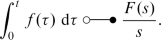
The Laplace transform is one of the standard tools used to analyze closed-loop control systems. In the scope of the book at hand, we deal only with the one-sided Laplace transform [3, 4], which is useful because processes can be described whereby signals are switched on at t = 0. Hence, the name “Laplace transform” will be used as a synonym for “one-sided Laplace transform.” Such a one-sided Laplace transform of a function f(t) with f(t) = 0 for t < 0 is given by
Here \(s =\sigma +j\omega\) is a complex parameter. It is obvious that the Laplace transform has a close relationship to the Fourier transform that is obtained for σ = 0 if only functions with f(t) = 0 for t < 0 are allowed. The real part of s is usually introduced to obtain convergence for a larger class of functions (please note that the Fourier transform of a sine or cosine function already leads to nonclassical Dirac pulses, as we saw in Sect. 2.1.5.3).
The Laplace transform F(s) of a function f(t) is an analytic function, and there is a unique correspondence between f(t) and F(s) if the classes of functions/distributions that are considered in the time domain and the Laplace domain are chosen accordingly [1, 4]. Since the integral in Eq. (2.25) exists only in some region of the complex plane, the Laplace transform is initially defined in only this region as well. If, however, a closed-form expression is obtained for the Laplace transform, e.g., a rational function, it is possible to extend the domain of definition by means of analytic continuation (cf. [5, Sect. 2.1]; [6, Sect. 10-9]; [7, Sect. 5.5.4]). Therefore, the Laplace transform F(s) should be defined as the analytic continuation of the function defined by Eq. (2.25). Apart from poles, a Laplace transform F(s) may thus be defined in the whole complex plane.
Like the Fourier transform, the Laplace transform is a linear transformation. If according to

we use the correspondence symbol again, the Laplace transform has the following properties (n is a positive integer, and a is a real number):
-
Laplace transform of a derivativeFootnote 1:

-
Derivative of a Laplace transform:

-
Laplace transform of an integral:
-
Shift theorems:

 (2.26)
 -
Convolution:
 (2.27)
 -
Scaling (a > 0):

-
Limits:
$$\displaystyle{ f(0+) =\lim _{s\rightarrow \infty }\left (s\;F(s)\right ), }$$$$\displaystyle{ f(\infty ):=\lim _{t\rightarrow \infty }f(t) =\lim _{s\rightarrow 0}\left (s\;F(s)\right ). }$$(2.28)Here f and its derivative must satisfy further requirements [4]. Before using the final-value theorem (2.28), for example, one should verify that the function actually converges for t → ∞.


Like the Fourier transform, the Laplace transform may also be generalized in order to cover distributions (i.e., generalized functions) [1]. Some common Laplace transforms are summarized in Table A.4 on p. 417.
2.3 Transfer Functions
Some dynamical systemsFootnote 2 may be described by the equation
In this case, X(s) and Y (s) are the Laplace transforms of the input signal x(t) and the output signal y(t), respectively. The Laplace transform H(s) is called the transfer function of the system. We discuss two specific input signals:
-
Let us assume that the input function x(t) is a Heaviside step function
In this case, the output is
$$\displaystyle{Y (s) = \frac{H(s)} {s}.}$$If we now apply Eq. (2.28), we obtain
$$\displaystyle{y(\infty ) =\lim _{s\rightarrow 0}H(s)}$$as the long-term (unit-)step response of the system.
-
If generalized functions are allowed, we may use x(t) = δ(t) as an input signal. In this case, the correspondence

leads to
$$\displaystyle{Y (s) = H(s),}$$which means that the transfer function H(s) corresponds to the impulse responseh(t) of the system. The final value of the response y(t) = h(t) is then given by
$$\displaystyle{y(\infty ) =\lim _{s\rightarrow 0}\left (s\;H(s)\right ).}$$


Let us assume that a system component is specified by the transfer function H(s). If we calculate the phase responseFootnote 3of this component according to \(\varphi (\omega ) = \measuredangle H(j\omega )\), the group delay can be defined by
Taking a dead-time element with \(H(s) = e^{-sT_{\mathrm{dead}}}\) (see shift theorem (2.26)) as an example, one obtains the frequency-independent, i.e., constant group delay
Hence, the dead-time element is an example of a device with linear phase response.
2.4 Mathematical Statistics
The results summarized in this chapter can be read in more detail in [8].
2.4.1 Gaussian Distribution
The Gaussian distribution (also called the normal distribution) is given by the probability density function
where \(\mu,\sigma \in \mathbb{R}\) with σ > 0 are specified. In order to ensure that f(x) is in fact a valid probability distribution, the equation
must hold. We show this by substituting
This leads to
By means of standard methods of mathematical analysis, one may show that
which actually leads to the result
For a given measurement curve that has the shape of a Gaussian distribution, one may use curve-fitting techniques to determine the parameters μ and σ. A simpler method is to determine the FWHM (full width at half maximum) value. According to Eq. (2.29), one-half of the maximum value is obtained for
The FWHM value equals twice this distance (one to the left of the maximum and one to the right of the maximum):
This formula may, of course, lead to less-accurate results than those obtained by the curve-fitting concept if zero line or the maximum cannot be clearly identified in the measurement data.
2.4.2 Probabilities
We now consider the area below the curve f(x) that is located to the left of \(x =\mu +\Delta x\), where \(\Delta x > 0\) holds. This area will be denoted by \(\Phi \):
It obviously specifies the probability that the random variableX is less than \(\mu +\Delta x\). By applying the same substitution as that mentioned above, one obtains
According to Fig. 2.1 we set
and get
The area D that is enclosed between \(\mu -\Delta x\) and \(\mu +\Delta x\) (see Fig. 2.2) can be calculated as follows:

Gaussian distribution

Gaussian distribution
Due to symmetry, we have
which leads to
Often, the area \(\Phi _{0}\) is considered, which is located between μ and \(\mu +\Delta x\):
This shows that D may also be written in the form
Some examples for these quantities are summarized in Table 2.2.
As an example, the table shows that the random variable is located in the confidence interval between μ − 2σ and μ + 2σ with a probability of 95. 45%.
2.4.3 Expected Value
Let X be a random variable with probability density function f(x). Then the expected value of the function g(X) is given by
It is obvious that the expected value is linear:
For g(X) = Xk, one obtains the kth moment:
By definition, the first moment is the mean of the random variable X. For the Gaussian distribution, we obtain
The term σ u in the parentheses leads to an odd integrand, so that this part of the integral vanishes.
Using Eq. (2.30), one obtains the mean
which is geometrically obvious.
If we always (not only for the Gaussian distribution) denote the mean by μ, then the kth central moment is given by
The second central moment is called the variance. For the Gaussian distribution, we obtain
With
an integration by parts yields
The first term on the right-hand side vanishes, and we get
The remaining integral is known from Eq. (2.30):
Hence we obtain
The variance is generally denoted by σ2 (not only for the Gaussian distribution), and its square root, the value σ, is called the standard deviation.
For a random sample with m values x1, x2, …, xm, one defines the sample mean
and the sample variance
For large samples, this value does not deviate much from \(\Delta x_{\mathrm{rms}}^{2}\), where the root mean square (rms) is definedFootnote 4 as
2.4.4 Unbiasedness
The individual values xk of a sample are the observed realizations of the random variables Xk that belong to the same distribution. Also,
is a random variable for which one may calculate the expected value. From E(Xk) = μ we obtain
which means that \(\bar{X}\) is an unbiased estimator of the mean value μ of the population. We now check whether the sample variance
is unbiased as well. We have
First of all, we need an expression for E(Xk2). For this purpose, we point out that all the random variables Xk belong to the same distribution, so that
holds. From E(Xk) = μ, we obtain
and
Now we analyze the second expression in Eq. (2.33), i.e., the expected value of
For independent random variablesX and Y, we have the equation
In our case, this is satisfied only for k ≠ l, which means for m − 1 terms. The term with k = l leads to the expected value E(Xk2) derived above. Therefore, we have
Finally, we calculate the expected value of
in an analogous way, obtaining
The results (2.34)–(2.36) may now be used in Eq. (2.33):
This shows that the sample variance is an unbiased estimator of the population variance. This is obviously not true for rms values. For large samples, however, this difference is no longer important.
We now calculate the variance of the sample mean \(\bar{X}\):
This shows that an estimate of the population mean from the sample mean becomes better as the sample size becomes larger.
2.4.5 Uniform Distribution
According to
we now calculate the variance of a uniform distribution:
In the last step, we substituted \(u = x-\mu\) to obtain
For large samples, we get
2.5 Bunching Factor
Let us consider a beam signal Ibeam(t) of a bunched beam as shown, for example, in Fig. 1.3 on p. 7. The bunching factor is defined as
i.e., it is the ratio of the average beam current to the maximum beam current (cf. Chao [9, Sect. 2.5.3.2, p. 131] or Reiser [10, Sect. 4.5.1, p. 263]). Obviously, the equation
holds, where TRF denotes the period.
Now one may replace the true shape of the beam current pulse by a rectangular one with the same maximum value. For \(-T_{\mathrm{RF}}/2 < t < T_{\mathrm{RF}}/2\), we then have
where we have assumed that the bunch is centered at t = 0. In this case, one has to choose a pulse width τ in such a way that the same average beam current is obtained:
Under these conditions, we obtain the expression
for the bunching factor.
We now assume that the beam current pulse has the shape of a Gaussian distribution. This is, of course, possible only if the pulses are significantly shorter than the period time TRF. Under this condition, the beam current will be close to zero before the next pulse starts.
Making use of Eq. (2.29), one may write Ibeam(t) in the form
We have
The average beam current is obtained using the above-mentioned approximation:
For the maximum current, we obtain
so that the bunching factor
is obtained. The equivalent length τ of a rectangular pulse is therefore
The two slopes of the rectangular pulse are therefore located at about ± 1. 25 σ. This leads to the conversion between the Gaussian bunch and the rectangular signal that is visualized in Fig. 2.3.

Gaussian beam signal
2.6 Electromagnetic Fields
We summarize in this section a few basic formulas that may be found in standard textbooks (cf. [11–17]). We begin with Maxwell’s equations in their integral form.
In the following, A denotes a two-dimensional domain, and V a three-dimensional domain. For a domain D (two- or threedimensional), ∂ D denotes its boundary (with mathematically positive orientation, if applicable).
Maxwell’s first equation (Ampère’s law) in the time domain is
where \(\vec{H}\) is the magnetizing field, \(\vec{J}\) the current density, and \(\vec{D}\) the electric displacement field.
Maxwell’s second equation in the time domain (Faraday’s law) reads
Here \(\vec{E}\) is the electric field, and \(\vec{B}\) is the magnetic field.
Maxwell’s third equation states that no magnetic charge exists:
The electric charge Q inside a three-dimensional domain V is determined by Maxwell’s fourth equation (Gauss’s law):
Here, ρq denotes the charge density.
The current through a certain region A is given by
and the voltage along a curve C is defined by
Please note that we use the same symbol for voltage and for threedimensional domains, but according to the context this should not lead to confusion.
In material bodies, the simplest relationships (linear isotropic media with relaxation times that are much smaller than the minimum time intervals of interest) between the field vectors are
The material parameters are the permittivity ε, the permeability μ, and the conductivity κ. In vacuum, and approximately also in air, we have
At least for fixed nonmoving domains A, we can write Eq. (2.39) in the form
where
is the magnetic flux through the domain A. This form is suitable for induction problems.
Based on the integral form of Maxwell’s equations presented above, one may derive their differential form if integral theorems are used:

Taking Eq. (2.44) into account, the divergence of Eq. (2.42) leads to the continuity equation
We will discuss the physical meaning of this equation in Sect. 2.9.
In certain cases (here we assume that domains are filled homogeneously with linear isotropic material), Maxwell’s equations may be solved by means of the vector potentialFootnote 5\(\vec{A}\), defined by
and the scalar potential\(\Phi \), defined by
both connected by the Lorenz gauge condition
Using these definitions, one obtains the wave equations

Here
denotes the speed of light in the material under consideration. The speed of light in vacuum is
For static problems, there is no time dependence of the fields, and according to Maxwell’s equations, electric and magnetic fields are therefore decoupled. In this case, the vector potential and the scalar potential also do not depend on time.
Equations (2.48) and (2.51) for homogeneous media thus reduce to
and the Poisson equation
respectively. This equation has to be solved for electrostatic problems.
2.7 Special Relativity
The primary objective of this section is to introduce the nomenclature that is used in this book. This nomenclature is close to that of the introductory text [17] (in German). In any case, the reader should consult standard textbooks on special (and general) relativity (cf. [11, 13, 18–20] in English or [14, 21–28] in German) for an extensive introduction. However, the remainder of the book can also be understood if the formulas presented in this section are regarded as given.
The speed of light c0 in vacuum has the same value in every inertial frame. Therefore, the equation of the wave front
in one inertial frame S (e.g., light flash at t = 0 at the origin of S) is transformed into a wave front equation
that has the same form in a different inertial frame \(\bar{S}\). Such transformation behavior is satisfied by the general Lorentz transformation. If one restricts generality in such a way that at t = 0, the origins of the two inertial frames are at the same position and that one frame \(\bar{S}\) moves with constant velocity v in the z-direction relative to the other frame S, then one obtains the special Lorentz transformation
The inverse transformation can be generated if the quantities with a bar (e.g., \(\bar{y}\)) are replaced by the same quantities without the bar (e.g., y) and vice versa. In that case, \(\bar{v} = -v\) has to be used (if \(\bar{S}\) moves with respect to S with velocity v in the positive z direction, S will move with respect to \(\bar{S}\) in the negative z direction), and c0 remains the same. This concept for generating inverse transformation formulas may also be applied to electromagnetic field quantities, whose transformation behavior is discussed below.
The square root in the denominator of Eqs. (2.58) and (2.59) is typical of expressions in special relativity. Therefore, the so-called Lorentz factors are defined:
Special relativity may be built up by defining so-called four-vectors and four-tensors. For example, the space coordinates are combined with the time “coordinate” in order to define the components of a four-vector that specifies the position in space-time:
Specific values of this four-vector can be interpreted as events. In combination with the special choice (signature)
for the metric tensor (i, k ∈ { 1, 2, 3, 4}), one obtains the desired transformation behavior of the wave front equation, because
which reproduces Eq. (2.55), is a tensor equation with a tensor of rank 0 (scalar) on the right-hand side. Here we use the Ricci calculus and Einstein’s summation convention. The special Lorentz transformation given above can now be reproduced by
which corresponds to the matrix equation
if the transformation coefficients
are chosen (i = row, k = column).
Similarly to the construction of the position four-vector, the vector potential and the scalar potential in electromagnetic field theory may be combined to form the electromagnetic four-potential \(\mathcal{A}\) according to
This, for example, allows one to write the Lorenz gauge condition (2.49) for free space in the form
of a tensor equation, where the vertical line indicates a covariant derivative, which—in special relativity—corresponds to the partial derivative because the metric coefficients are constant.
The four-current density\(\mathcal{J}\) is defined by
so that the tensor equation
represents the continuity equation (2.46). The transformation law obviously yields
With \(\vec{v} = v\vec{e}_{z}\) defining the parallel direction ∥ , this may be written in the generalized form
The electromagnetic field tensor may be defined as
while its counterpart for the other field components in Maxwell’s equations may be defined as
where i specifies the row, and k the column. The introduction of these four-vectors and four-tensors allows one to write Maxwell’s equations asFootnote 6
so that their form remains the same if a Lorentz transformation from one inertial frame to a different one is performed. This form invariance of physical laws is called covariance. The covariance of Maxwell’s equations implies the constancy of c0 in different inertial frames, since c0 is a scalar quantity, a tensor of rank 0. Because \(\mathcal{B}^{ik}\) and \(\mathcal{H}^{ik}\) are tensors of rank 2, they are transformed according to the transformation rule
Taking the second transformation rule as an example, this may be translated into the matrix equation
A long but straightforward calculation then leads to the transformation laws for the corresponding field components:
The generalized form is
The remaining transformation laws are obtained analogously:
In the scope of this book, there is no need to develop the theory further. Nor do we discuss such standard effects as time dilation, Lorentz contraction, and the transformation of velocities. However, we need some relativistic formulas for mechanics.
The definition of the Lorentz force (1.1) is valid in special relativity—it corresponds to a covariant equation (the charge Q is invariant; it is a scalar quantity).
Also, the equation
with the momentum definition
based on the velocity
still holds. However, the mass m is not invariant. Only the rest massm0 is a tensor of rank zero, i.e., a scalar:
Please note that we strictly distinguish between the velocities v and u and also between the related Lorentz factors. The velocity \(\vec{v} = v\;\vec{e}_{z}\) is defined as the relative velocity of the inertial frame \(\bar{S}\) with respect to the inertial frame S, i.e., the velocity between these two reference frames. The velocity \(\vec{u}\) is the velocity of a particle measured in the first inertial frame S. Consequently, \(\vec{\bar{u}}\) is the velocity of the same particle in the inertial frame \(\bar{S}\). If it is clear what is meant by a certain Lorentz factor, one may, of course, omit the subscript.
The total energy of a particle with velocity \(\vec{u}\) is given by
Consequently, the rest energy is obtained for \(\vec{u} = 0\), which leads to γu = 1:
Therefore, the kinetic energy is
Using the Lorentz factors, one may write the momentum in the form
leading to the absolute value
Here we used the definition
If we have a look at Eqs. (2.89)–(2.91), we observe that γ is related to the energy, the product β γ to the momentum, and β corresponds to the velocity. It is often helpful to keep this correspondence in mind when complicated expressions containing a large number of Lorentz factors are evaluated. One should also keep in mind that when one of the expressions β, γ, β γ is known, the others are automatically fixed as well.
This is why we can also convert expressions for relative deviations into each other. For example, we may calculate the time derivative of
as follows:
Here we can use the relation
which follows directly from Eq. (2.92):
Expressions of this type are very helpful, because they can be translated as follows:
This conversion is possible if the relative change in the quantities is sufficiently small. In the example presented here, one can see directly that a velocity deviation of 1% is transformed into an energy deviation of 3% if γ = 2 holds.
As a second example, we can calculate the time derivative of Eq. (2.93):
This can be translated into
Relations like these are summarized in Table 2.3.
In accelerator physics and engineering, specific units that contain the elementary charge e are often used to specify the energy of the beam. This is due to the fact that the energy that is gained by a chargeFootnote 7Q = zqe is given by formula (1.2),
An electron that passes a voltage of V = 1 kV will therefore lose or gain an energy of 1 keV, depending on the orientation of the voltage. We have only to insert the quantities into the formula without converting e into SI units. In order to convert an energy that is given in eV into SI units, one simply has to insert \(e = 1.6022 \cdot 10^{-19}\,\mathrm{C}\), so that \(1\,\mathrm{eV} = 1.6022 \cdot 10^{-19}\,\mathrm{J}\) holds.
Also, the rest energy of particles is often specified in eV. For example, the electron rest mass \(m_{\mathrm{e}} = 9.1094 \cdot 10^{-31}\,\mathrm{kg}\) corresponds to an energy of 510. 999 keV.
As we saw above, the energy directly determines the Lorentz factors and the velocity. Therefore, it is desirable to specify the energy in a unit that directly corresponds to a certain velocity. Due to
a kinetic energy of 1 MeV leads to different values for γ if different particle rest masses m0 are considered. This is why one introduces another energy unit for ions. An ion with mass number A has rest mass
where \(m_{\mathrm{u}} = 1.66054 \cdot 10^{-27}\,\mathrm{kg}\) denotes the unified atomic mass unit (as mentioned below, Ar differs slightly from A). Therefore, one obtains
If the value on the right-hand side is specified now, γ is determined in a unique way, since mu and c0 are global constants. As an example, an ion beam with a kinetic energy ofFootnote 8 11. 4 MeV∕u corresponds to γ = 1. 0122386 and β = 0. 15503. We do not need to specify the ion species.
Ions are usually specified by the notation
Here A is the (integer) mass number, i.e., the number of nucleons (protons plus neutrons); Z is the atomic number, which equals the number of protons and identifies the element. For example,
indicates a uranium ion that has \(A - Z = 146\) neutrons. Different uranium isotopesFootnote 9 exist with a different number of neutrons. The number of protons however, is the same for all these isotopes. Therefore, Z is redundant information that is already included in the element name. In the last example, the uranium atom has obviously lost 28 of its 92 electrons, leading to the charge number zq = 28.
The unified atomic mass unit mu is defined as 1∕12 of the mass of the atomic nucleus612C. For different ion species and isotopes, the mass is not exactly an integer multiple of mu (reasons: different mass of protons and neutrons, relativistic mass defect due to binding energy). For238U, for example, one has Ar = 238. 050786, which approximately equals A = 238.
2.8 Nonlinear Dynamics
A continuous dynamical system of first order may be described by the following first-order ordinary differential equation (ODE):
The state of a dynamical system of order n is represented by the values of n variables x1, x2, …, xn, which may be combined into a vector \(\vec{r} = (x_{1},x_{2},\ldots,x_{n})\). Hence, a dynamical system of order n is described by the system of ordinary differential equations
One should note that the system of ODEs is still of order 1, but of dimension n. Such a system is called autonomous when \(\vec{v}(\vec{r},t)\) does not depend on the timeFootnote 10t, i.e., when
holds. The next sections will show that Eq. (2.94), which may look very simple at first sight, includes a huge variety of problems.
2.8.1 Equivalence of Differential Equations and Systems of Differential Equations
Let us consider the nth-order linear ordinary differential equation
with dimension 1. One sees that by means of the definitions
it may be converted into the form
which is equivalent to the standard form
If b and all the ak do not depend on time (ODE of order n with constant coefficients), then \(\vec{v}\) will also not depend on time explicitly, so that an autonomous system is present.
Although the vector field \(\vec{v}\) is called a velocity function, it does not always correspond to a physical velocity. As already mentioned, the variable t is not necessarily the physical time. However, we will use this notation because the reader may always interpret these variables in terms of the mechanical analogy, which may help to understand the physical background.
The above-mentioned equivalence is also valid for nonlinear ODEs of the form
whereFootnote 11F ∈ C1. Also here, we may use
to obtain the standard form
An autonomous system results when F and \(\vec{v}\) do not explicitly depend on the time variable t.
2.8.2 Autonomous Systems
Hereinafter, we will consider only autonomous systems if a time dependence is not stated explicitly.
2.8.2.1 Time Shift
An advantage of autonomous systems is the fact that if a solution y(t) of
is known, then \(z(t) = y(t - T)\) will also be a solution if T is a constant time shift. This can be shown as follows:
The solution y(t) is the first component of the vector \(\vec{r}(t)\) that satisfies the differential equationFootnote 12
Therefore, z(t) is the first component of the vector
We obtain
One sees that \(\vec{r}_{\mathrm{shift}}(t)\) satisfies the system of ODEs in the same way as \(\vec{r}(t)\) does. Due to the equivalence with the differential equation of order n, z(t) will be a solution as well.
This explains, for instance, why sin(ω t) must be a solution of the homogeneous differential equation
if one knows that cos(ω t) is a solution. This ODE is autonomous, and these two solutions differ only by a time shift.
2.8.2.2 Phase Space
The phase space may be defined as the continuous space of all possible states of a dynamical system. In our case, the dynamical system is described by an autonomous system of ordinary differential equations.
The graphs of the solutions \(\vec{r}(t)\) of the differential equation are the integral curves or solution curves in the n-dimensional phase space. Such an integral curve contains the dependence on the parameter t (which is usually but not necessarily the time). A different parameterization therefore leads to a different integral curve.
The set of all image points of the map \(t\mapsto \vec{r}(t)\) is called the orbit. An orbit does not contain dependence on the parameter t. A different parameterization therefore leads to the same orbit, since the same image points are obtained simply by a different value of the parameter t.
Different orbits of an autonomous system are often drawn in a phase portrait, which may be defined as the set of all orbits.
2.8.3 Existence and Uniqueness of the Solution of Initial Value Problems
The standard form
has the advantage that it can be solved numerically according to the (explicit) Euler method:
It is obvious that by defining the initial condition
the states
of the system at different times can be derived iteratively for k > 0 (\(k \in \mathbb{N}\)). The states of the system may be calculated for both future times t > t0 and past times t < t0 in a unique way by selecting the sign of \(\Delta t\). However, this is possible only in a certain neighborhood around t0, as we will see in the next sections.
It is obvious that by defining \(\vec{r}_{0}\), n scalar initial conditions are required to make the solution unique.
2.8.3.1 Existence of a Local Solution
The existence of a solution is ensured by the following theorem:
Theorem 2.1 (Peano).
Consider an initial value problem
with a continuous \(\vec{v}: D \rightarrow \mathbb{R}^{n}\) on an open set \(D \subset \mathbb{R}^{n+1}\) . Then there exists \(\alpha (\vec{r}_{0},t_{0}) > 0\) such that the initial value problem has at least one solution in the interval \([t_{0}-\alpha,t_{0}+\alpha ]\) .
(See Aulbach [29, Theorem 2.2.3].)
Remark.
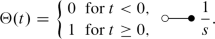
We may easily see that \(\vec{v}\) must be continuous. If we choose \(v = \Theta (t)\) (Heaviside step function) in the one-dimensional case, we immediately see that the derivative \(\frac{\mathrm{d}r} {\mathrm{d}t}\) is not defined at t = 0. Therefore, in the scope of classical analysis, we have to exclude functions that are not continuous. In the scope of distribution theory, the solution \(r = t\;\Theta (t)\) is obvious.
2.8.3.2 Uniqueness of a Local Solution
Uniqueness can be ensured if the vector field \(\vec{v}\) satisfies a Lipschitz condition or if it is continuously differentiable.
Definition 2.2.
The vector function \(\vec{v}(\vec{r},t): D \rightarrow \mathbb{R}^{n}\) (\(D \subset \mathbb{R}^{n+1}\) open) is said to satisfy a global Lipschitz condition on D with respect to \(\vec{r}\) if there is a constant K > 0 such that for all \((\vec{r}_{1},t),(\vec{r}_{2},t) \in D\), the condition
holds. Instead of saying that a function satisfies a global Lipschitz condition, one also speaks of a function that is Lipschitz continuous.
(Cf. Aulbach [29, Definition 2.3.5] and Perko [30, p. 71, Definition 2].)
Definition 2.3.
The vector function \(\vec{v}(\vec{r},t): D \rightarrow \mathbb{R}^{n}\) (\(D \subset \mathbb{R}^{n+1}\) open) is said to satisfy a local Lipschitz condition on D with respect to \(\vec{r}\) if for each \((\vec{r}_{0},t_{0}) \in D\), there exist a neighborhood \(U_{(\vec{r}_{0},t_{0})} \subset D\) of \((\vec{r}_{0},t_{0})\) and a constant K > 0 such that for all \((\vec{r}_{1},t),(\vec{r}_{2},t) \in U_{(\vec{r}_{0},t_{0})}\), the condition
holds. Instead of saying that a function satisfies a local Lipschitz condition, one also speaks of a function that is locally Lipschitz continuous.
(Cf. Aulbach [29, Definition 2.3.5], Wirsching [31, Definition 3.4], and Perko [30, p. 71, Definition 2].)
In other words, the function satisfies a local Lipschitz condition if for every point, we can find a neighborhood such that a “global” Lipschitz condition holds in that neighborhood.
Example.
The function f(x) = x2 is locally Lipschitz continuous, but it is not Lipschitz continuous.
Theorem 2.4 (Picard–Lindelöf).
Consider the initial value problem
with continuous \(\vec{v}: D \rightarrow \mathbb{R}^{n}\) ( \(D \subset \mathbb{R}^{n+1}\) open). Suppose that the vector function \(\vec{v}(\vec{r},t)\) is locally Lipschitz continuous with respect to \(\vec{r}\) . Then there exists \(\alpha (\vec{r}_{0},t_{0}) > 0\) such that the initial value problem has a unique solution in the interval \([t_{0}-\alpha,t_{0}+\alpha ]\) .
(See Aulbach [29, Theorem 2.3.7].)
Every locally Lipschitz continuous function is also continuous.
Every continuously differentiable function satisfies a local Lipschitz condition, i.e., is locally Lipschitz continuous (Aulbach [29, p. 77], Arnold [32, p. 279], Perko [30, lemma on p. 71]).
Therefore, the Picard–Lindelöf theorem may simply be rewritten for continuously differentiable functions instead of locally Lipschitz continuous functions (Perko [30, p. 74]: “The Fundamental Existence-Uniqueness Theorem,” Guckenheimer/Holmes [33, Theorem 1.0.1]).
2.8.3.3 Maximal Interval of Existence
One may try to make the solution interval larger by using the endpoint of the solution interval as a new initial condition. If this strategy is executed iteratively, one obtains the maximal interval of existence. It is an open interval (cf. [30, p. 89, Theorem 1]). The maximal interval of existence does not necessarily correspond to the full real time axis. Further requirements are necessary to ensure this.
2.8.3.4 Global Solution
A continuously differentiable vector field \(\vec{v}\) is called complete if it induces a global flow,Footnote 13 i.e., if its integral curves are defined for all \(t \in \mathbb{R}\).
Every differentiable vector field with compact support is complete.
The following theorem shows that certain restrictions on the “velocity” \(\vec{v}(\vec{r})\) are sufficient for completeness:
Theorem 2.5.
Let the vector function \(\vec{v}(\vec{r})\) with \(\vec{v}: D \rightarrow \mathbb{R}^{n}\) ( \(D \subset \mathbb{R}^{n}\) open) be continuously differentiable and linearly bounded with K,L ≥ 0:
Then the initial value problem
has a global flow.
(Cf. Zehnder [34, Proposition IV.3, p. 130], special form of Theorem 2.5.6, Aulbach [29].)
According to Amann [35, Theorem 7.8], the solution will then be bounded for finite time intervals.
Like many other authors, Perko [30, p. 188, Theorem 3] requires that \(\vec{v}(\vec{r})\) satisfy a global Lipschitz condition
for arbitrary \(\vec{r}_{1},\vec{r}_{2} \in \mathbb{R}^{n}\). For \(\vec{r}_{2} = 0\), this leads to linear boundedness, as one may show by means of the reverse triangle inequality, but it is a stronger condition.
Example.
The ODE
is obviously satisfied for
This solution may be found by separation of variables. An arbitrary initial condition y(0) = y0 may be satisfied if the shifted solution
is considered. In any case, however, the solution curve reaches infinity while t is still finite. The “vector” field \(v(y) = 1 + y^{2}\) is not complete, and it is obviously not linearly bounded.
If we simplify the results of this section, we may summarize them as follows:
-
The existence of a local solution is ensured by continuity of \(\vec{v}\).
-
Local Lipschitz continuity ensures uniqueness of the solution. If \(\vec{v}\) is continuously differentiable, uniqueness is also guaranteed.
-
If linear boundedness of \(\vec{v}\) is required in addition, a global solution/global flow exists.
For the sake of simplicity, we will consider only complete vector fields in the following.
2.8.3.5 Linear Systems of Ordinary Differential Equations
For linear systems of differential equations with
where A is a quadratic matrix with real constant elements, we may use the matrix norm:
Therefore, the conditions of Theorem 2.5 are satisfied, and a unique solution with a global flow exists. One may specifically use the Frobenius norm
which is compatible with the Euclidean norm
of a vector, so that
holds.
2.8.4 Orbits
Two distinct orbits of an autonomous system do not intersect. In order to prove this, we assume the contrary. Suppose that two distinct orbits defined by \(\vec{r}_{1}(t)\) and \(\vec{r}_{2}(t)\) intersect according to
Please note that the intersection point may be reached for different values t1 and t2 of the parameter t, since we require only that the orbits (i.e., the images of the solution curves) intersect. As shown in Sect. 2.8.2.1,
is also a solution of the differential equation. Therefore, we have
Hence \(\vec{r}_{\mathrm{shift}}(t)\) and \(\vec{r}_{2}(t)\) satisfy the same initial conditions at the time t2. This means that the solution curves \(\vec{r}_{\mathrm{shift}}(t)\) and \(\vec{r}_{2}(t)\) are identical.
Since \(\vec{r}_{1}(t)\) is simply time-shifted with respect to \(\vec{r}_{\mathrm{shift}}(t) =\vec{ r}_{2}(t)\), the images, i.e., the orbits, will be identical. This means that two orbits are completely equal if they have one point in common.
In other words, each point of phase space is crossed by only one orbit.
2.8.5 Fixed Points and Stability
Vectors \(\vec{r} =\vec{ r}_{\mathrm{F}}\) for which
holds are called fixed points (or equilibrium points or stationary points or critical points) of the dynamical system given by
This nomenclature is obvious, since a particle that is initially located at
will stay there forever:
Definition 2.6.
A fixed point of an autonomous dynamical system is called an isolated fixed point or a nondegenerate fixed point if an environment of the fixed point exists that does not contain any other fixed points.
(Cf. Sastry [36, Definition 1.4, p. 13], Perko [30, Definition 2, p. 173].)
We now define the stability of fixed points according to Lyapunov.
Definition 2.7.
A fixed point is called stable if for every neighborhood U of \(\vec{r}_{\mathrm{F}}\), another neighborhood V ⊂ U of \(\vec{r}_{\mathrm{F}}\) exists such that a trajectory starting in V at t = t0 will remain in U for all t ≥ t0 (see Fig. 2.4). Otherwise, the fixed point is called unstable.

Stability (left) and asymptotic stability (right) of a fixed point
Please note that it is usually necessary to choose V smaller than U, because the shape of the orbit may cause the trajectory to leave U for some starting points in U even if \(\vec{r}_{\mathrm{F}}\) is stable.
Definition 2.8.
A stable fixed point \(\vec{r}_{\mathrm{F}}\) is called asymptotically stable if a neighborhood U of \(\vec{r}_{\mathrm{F}}\) exists such that for every trajectory that starts at t = t0 in U, the following equation holds:
(See, e.g., Perko [30, Definition 1, p. 129].)
Definition 2.9.
A function \(L(\vec{r})\) with L ∈ C1 and \(L: U \rightarrow \mathbb{R}\) (\(U \subset \mathbb{R}^{n}\) open) is called a Lyapunov function for the fixed point \(\vec{r}_{\mathrm{F}}\) of the autonomous system
if
and
hold in a neighborhood U ⊂ D of \(\vec{r}_{\mathrm{F}}\).
A Lyapunov function is called a strict Lyapunov function if
holds.
(Cf. Perko [30, p. 131, Theorem 3], La Salle/Lefschetz [37, Sect. 8], Guckenheimer/Homes [33, Theorem 1.0.2].)
Theorem 2.10.
If a Lyapunov function for a fixed point \(\vec{r}_{\mathrm{F}}\) of an autonomous system exists, then this fixed point \(\vec{r}_{\mathrm{F}}\) is stable. If a strict Lyapunov function exists, then this fixed point \(\vec{r}_{\mathrm{F}}\) is asymptotically stable.
(Cf. Perko [30, p. 131, Theorem 3].)
It is easy to see that this theorem is valid. For two-dimensional systems with the particle trajectory \(\vec{r}(t) = x(t)\;\vec{e}_{x} + y(t)\;\vec{e}_{y}\), we obtain, for example,Footnote 14
If this expression is negative, the strict Lyapunov function will decrease while the particle continues on its path. Since the minimum of the Lyapunov function is obtained for \(\vec{r}_{\mathrm{F}}\), it is clear that the particle will move toward the fixed point.
Similar reasoning applies for a Lyapunov function that is not strict. In this case, the particle cannot move away from the fixed point, because the Lyapunov function does not increase. However, it will not necessarily get closer to the fixed point.
2.8.6 Flows of Linear Autonomous Systems
Having shown above that a linear autonomous system possesses a global flow, we shall now compute this flow. If an autonomous system of order n is linear, we may describe it by
with
where A is a quadratic n × n matrix with real constant elements. The ansatz
leads to
or
For nontrivial solutions \(\vec{w}\neq 0\), the condition
is necessary, which determines the eigenvaluesλ. For the sake of simplicity, we now assume that all n eigenvalues are distinct and that there is one eigenvector belonging to each eigenvalue (A is diagonalizable in this case). The overall solution of the homogeneous system of ODEs may then be written in the form
where \(\vec{w}_{k}\) denotes the eigenvector that belongs to the eigenvalue λ = λk and where the Ck are constants. For the initial condition at t = 0, we therefore have
According to Eq. (2.95), the solution is obviously asymptotically stable if and only if
holds for all \(k \in \{ 1,2,\ldots,n\}\), since only then does
hold for arbitrary initial conditions. In this case, \(\vec{r} = 0\) is an asymptotically stable fixed point.
Now we raise the question whether further fixed points exist. This is the case for
with
i.e., only for
In Sect. 2.8.8, we will see that this is the condition for a degenerate, i.e., nonisolated, fixed point (see Definition 2.6, p. 59).
Let us now determine a map that transforms an initial value \(\vec{r}_{0}\) into a vector \(\vec{r}(t)\) that satisfies the linear autonomous system of ODEs
The overall solution
with eigenvectors
may, due to
be written as the matrix equation
We define
(matrix of the eigenvectors),
and
Hence we have
For t = 0, we obtain
Due to
the definition
makes sense. Finally, we obtain
Using the matrix exponential function
one also writes
This equation obviously determines the global flow (Guckenheimer [33, Eqn. (1.1.9), p. 9]) if the following definition is used:
Definition 2.11.
A (global) flow is a continuous map \(\Phi: \mathbb{R} \times D \rightarrow D\), which transforms each initial value \(\vec{r}(0) =\vec{ r}_{0} \in D\) (\(D \subset \mathbb{R}^{n}\) open) into a vector \(\vec{r}(t)\) (\(t \in \mathbb{R}\)) satisfying the following conditions:
Here we have defined \(\Phi _{t}(\vec{r}):= \Phi (t,\vec{r})\).
(Cf. Wiggins [38, Proposition 7.4.3, p. 93], Wirsching [31, Definition 8.6], Amann [39, p. 123/124].)
The interpretation of this definition is simple: If no time passes, one remains at the same point. Instead of moving from a first point to a second one in the time span t2 and then from this second one to a third one in a time span t1, one may go directly from the first to the third in the time span t1 + t2.
Remark.
-
A flow (also called a phase flow) is called a global flow if it is defined for all \(t \in \mathbb{R}\) (as in Definition 2.11), a semiflow if it is defined for all \(t \in \mathbb{R}^{+}\), and a local flow if it is defined for t ∈ I (open interval I with 0 ∈ I).
-
For semiflows and local flows, Definition 2.11 has to be modified.
-
In the modern mathematical literature, a dynamical system is defined as a flow. In our introduction, however, the dynamical system was initially described by an ODE, and the corresponding velocity vector field induced the flow.
Final remark: If the matrix A does not possess n linearly independent eigenvectors, then no diagonalization is possible, in which this case generalized eigenvectors may be used (cf. Guckenheimer [33, p. 9]). These are defined by
and may be used to transform any quadratic matrix A into Jordan canonical form (cf. Burg et al. [40, vol. II, p. 293] or Perko [30, Sect. 1.8]). As the formula shows, eigenvectors are also generalized eigenvectors (for p = 1).
2.8.7 Topological Orbit Equivalence
In this section, we shall define what it means to say that two vector fields are topologically orbit equivalent. Of course, the term topological orbit equivalence will include the case that the two vector fields can be transformed into each other by a simple rotation.
In order to simplify the situation even further, we assume that the two vector fields are given by
and
where A and B are quadratic matrices.
If one vector field can be obtained as a result of rotating the other one, there must be a rotation matrix M such that
holds. Now \(\vec{v}_{2}\) depends on \(\vec{r}_{1}\). In order to make \(\vec{v}_{2}\) dependent on \(\vec{r}_{2}\), we must rotate the coordinates in the same way as the vector field (see Fig. 2.5):
Hence, we obtain
Since M is invertible as a rotation matrix, the matrix
describes the well-known similarity transformation that may also be written in the form
A similarity transformation, however, is usually written in the form
so that we have to define \(\tilde{M} = M^{-1}\) here.

Rotation of a vector field
Now we observe that two orbits can be identical even though the corresponding solution curves are parameterized in a different way.
A flow for Eq. (2.100) will be denoted by
and a flow for Eq. (2.101) by
In order to transform the orbits of these flows into each other, the starting points must be mapped first:
Our requirement that different parameterizations be allowed for both solution curves may be translated as follows: For every time t1, there is a time t2 such that
and therefore
holds. This formula must be included in the general definition of topological orbit equivalence if rotations are to be allowed as topologically equivalent transformations.
The previous considerations make the following definition transparent:
Definition 2.12.
Two C1 vector fields \(\vec{v}_{1}(\vec{r}_{1})\) and \(\vec{v}_{2}(\vec{r}_{2})\) are called topologically orbit equivalentFootnote 15 if a homeomorphism h exists such that for every pair \(\vec{r}_{10}\), t1, there exists t2 such that
holds. Here, the orientation of the orbits must be preserved. If in addition, the parameterization by time is preserved, the vector fields are called topologically conjugate. In this definition, \(\Phi _{t}^{\vec{v}}\) denotes the flow that is induced by the vector field \(\vec{v}\).
(Cf. Sastry [36, Definition 7.18, p. 303], Wiggins [38, Definition 19.12.1, p. 346], Guckenheimer [33, p. 38, Definition 1.7.3].)
Remark.
A homeomorphism is a continuous map whose inverse map exists and is also continuous. The fact that a homeomorphism is used as a generalization of the rotation matrix, used as an example above, leads to the following features:
-
Not only linear maps are allowed, but also nonlinear ones.
-
The requirement that the map be continuous guarantees that neighborhoods of a point are mapped to neighborhoods of its image point. Therefore, the orbits are deformed but not torn apart. Two examples for topological orbit equivalence are shown in Fig. 2.6.
Fig. 2.6 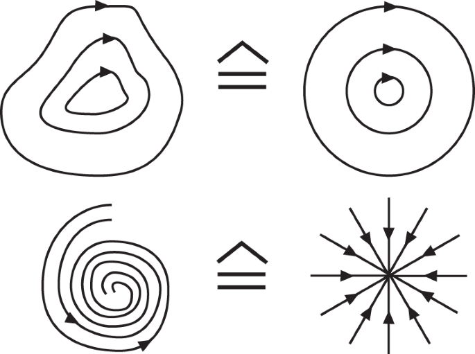
Examples of topological orbit equivalence

The fact that the validity of Eq. (2.104) is required for each initial point ensures that all orbits are transformed into each other. Hence, the entire phase portraits will be equivalent.
The preservation of the orientation may be checked by means of a continuously differentiable function \(t_{2}(\vec{r}_{10},t_{1})\) with \(\frac{\partial t_{2}} {\partial t_{1}} > 0\) (cf. Perko [30, Sect. 3.1, Remark 2, p. 183/184]).
Please note that different authors use slightly different definitions. In cases of doubt, one should therefore check the relevant definitions thoroughly.
Let us now consider the case that a vector field \(\vec{v}(\vec{r}) = A \cdot \vec{ r}\) is given by a real n × n matrix A and that we want to check whether this vector field is topologically orbit equivalent to a simpler vector field. Often, diagonalization is possible. This case will be discussed in the following.
Remark.
-
In case diagonalization is not possible, it is always possible to transform the matrix into Jordan canonical form.
-
Diagonalization of an n × n matrix is possible if and only if for each eigenvalue, the algebraic multiplicity (multiplicity of the zeros of the characteristic polynomial) equals the geometric multiplicity (number of linearly independent eigenvectors).
-
Diagonalization of an n × n matrix is possible if and only if it possesses n linearly independent eigenvectors.
-
Diagonalization is possible for every symmetric matrix with real elements.
Consider a matrix A for which diagonalization is possible. We will show now that the diagonal matrixFootnote 16
does in fact lead to a topologically orbit equivalent vector field. Here, \(\tilde{M} = M^{-1} = X_{A}(0)\) denotes the matrix of the n eigenvectors of A. These are linearly independent, since diagonalization of A is possible (cf. Burg/Haf/Wille [40, vol. II, p. 280, Theorem 3.52]).
According to Eqs. (2.98) and (2.99), the flows are given by
for A and by
for B. In our case, the homeomorphism h is given by the matrix M. We therefore obtain
On the other hand,
holds. We see that these expressions are equal for every initial vector \(\vec{r}_{10}\) if
or
is valid. Due to Eq. (2.97), we know that
and
hold, so that the equation
has to be verified. Since B is a diagonal matrix, the Cartesian unit vectors are eigenvectors, so that
is valid. Therefore, we have only to check whether
is true. Since the eigenvalues of A and B are equal due to diagonalization, we obtain
Here we had only to set t2 = t1. We have shown that diagonalization leads to topologically orbit equivalent vector fields.
2.8.8 Classification of Fixed Points of an Autonomous Linear System of Second Order
The considerations presented above indicate that a similarity transformation
always leads to topologically orbit equivalent vector fields. Every similarity transformation leaves the eigenvalues unchanged (cf. Burg/Haf/Wille [40, vol. II, p. 272, 3.17]). This leads us to the assumption that the eigenvalues of a matrix at least influence the topological properties of the related vector field. Therefore, the eigenvalues are now used to characterize the fixed points.
We calculate the eigenvalues of a two-dimensional matrix
with constant real elements. This leads to
Hence, we obtain
with
We now try to distinguish as many cases as possible:
-
1.
Both eigenvalues are real (C ≥ 0).
-
(a)
Both are positive
-
(i)
λ1 > λ2 > 0
-
(ii)
λ1 = λ2 > 0
-
(i)
-
(b)
Both are negative
-
(i)
λ1 < λ2 < 0
-
(ii)
λ1 = λ2 < 0
-
(i)
-
(c)
One is positive, one is negative: λ1λ2 < 0
-
(d)
One equals 0 (λ1 = 0):
-
(i)
λ2 > 0
-
(ii)
λ2 < 0
-
(iii)
λ2 = 0
-
(i)
-
(a)
-
2.
Imaginary eigenvalues: C < 0, B = 0, \(\lambda _{2} = -\lambda _{1}\)
-
3.
Complex eigenvalues: C < 0, λ1 = λ2∗
-
(a)
B = Re{λ} < 0
-
(b)
B = Re{λ} > 0
-
(a)
Hence we have found 11 distinct cases. If one eigenvalue is zero, then Eq. (2.106) leads to
As we will show now, this means in general that one row is a multiple of the other row, which contains the special case that one or both rows are zero.
If we now assume that the second row is a multiple of the first one,
we obtain the following condition for the eigenvalues:
This shows that at least one eigenvalue is zero. The same can be shown for the case that the first equation is a multiple of the second one. Since one eigenvalue is 0, the relation
leads to
In conclusion, the following statements for our two-dimensional case are equivalent:
-
det A = 0.
-
One row of A is a multiple of the other row.
-
At least one eigenvalue is 0.
The following general theorem holds:
Theorem 2.13.
The following statements for a quadratic matrix A are equivalent:
-
The quadratic matrix A is regular.
-
All row vectors (or column vectors) of A are linearly independent.
-
det A ≠ 0.
-
All eigenvalues of A are nonzero.
-
A is invertible.
In our two-dimensional case, the statement that for det A = 0, one row is a multiple of the other one means that the equation \(\vec{v}(\vec{r}) = A \cdot \vec{ r} = 0\) is satisfied along a line through the origin or even everywhere. Hence, we have an infinite number of fixed points that are not separated from each other. In this case, we speak of degenerate fixed points (see Definition 2.6 on p. 59). This case will henceforth be excludedFootnote 17 (case 1.d), so that the number of relevant cases is reduced from 11 to 8. According to the behavior of the vector field in the vicinity of the fixed point \(\vec{r}_{\mathrm{F}} = 0\), the fixed points are named as follows:
-
1.
Both eigenvalues are real (C ≥ 0).
-
(a)
Both positive
-
(i)
λ1 > λ2 > 0: unstable node
-
(ii)
λ1 = λ2 > 0: unstable improper node or unstable star
-
(i)
-
(b)
Both negative
-
(i)
λ1 < λ2 < 0: stable node
-
(ii)
λ1 = λ2 < 0: stable improper node or stable star
-
(i)
-
(c)
One positive, one negative: λ1λ2 < 0: saddle point
-
(a)
-
2.
Imaginary eigenvalues: C < 0, B = 0, \(\lambda _{2} = -\lambda _{1}\): center or elliptic fixed point
-
3.
Complex eigenvalues: C < 0, λ1 = λ2∗
-
(a)
Re{λ} < 0: stable spiral point or stable focus
-
(b)
Re{λ} > 0: unstable spiral point or unstable focus
-
(a)
The classification of fixed points is summarized in Table 2.4 on p. 74 (cf. [29, 42, 43]). As the table shows, not only the eigenvalues can be used to characterize the fixed points. In the column “Topology”, the numbers in parentheses denote the quantity of eigenvalues with positive real part. The column “Topology” also contains the so-called index in brackets. In order to calculate the index, one considers a closed path around the fixed point with an orientation that is mathematically positive. Now one checks how many revolutions the vectors of the vector field perform while “walking” on the path. If, e.g., the vectors of the vector field also perform one revolution in mathematically positive orientation, the index is + 1. If the vector field rotates in opposite direction, the index is − 1.
Figures 2.7, 2.8, 2.9, 2.10, 2.11, and 2.12 on p. 75 and 76 show how orbits in the vicinity of the fixed point look in principle for each type of fixed point. In case the fixed point is a stable node, star, or spiral point, the orientation of the solution curves will be towards the fixed point in the middle; in case of an unstable node, star, or spiral point, all solution curves will be directed outwards. Each picture is just an example; in the specific case under consideration the orbits may of course be deformed significantly.

Center

Node with two tangents

Node with one tangent

Star

Spiral point

Saddle point
2.8.9 Nonlinear Systems
Consider the nonlinear autonomous system
with the initial condition
where \(\vec{v}(\vec{r}) \in C^{2}\) has a fixed point \(\vec{r}_{\mathrm{F}}\) with
As the results summarized in this section show, the linearization
of the system (2.109), where \(A = D\vec{v}(\vec{r}_{\mathrm{F}})\) is the Jacobian matrixFootnote 18 at \(\vec{r} =\vec{ r}_{\mathrm{F}}\), is a powerful tool for analyzing a nonlinear system in the vicinity of its fixed points. Please note that \(\vec{r} = 0\) in Eq. (2.110) corresponds to \(\vec{r} =\vec{ r}_{\mathrm{F}}\) in Eq. (2.109), i.e., the fixed point of the nonlinear system was shifted to the origin of the linearized system.
Theorem 2.14.
Consider the nonlinear system (2.109) with the linearization (2.110) at a fixed point\(\vec{r}_{\mathrm{F}}\). If A is nonsingular, then the fixed point\(\vec{r}_{\mathrm{F}}\)is isolated (i.e., nondegenerate).
(See Sastry [36, Proposition 1.5, p. 13], Perko [30, Definition 2, p. 173].)
If one or more eigenvalues of the Jacobian matrix are zero, the fixed point is a degenerate fixed point. This is the generalization of the linear case.
Definition 2.15.
A fixed point is called a hyperbolic fixed point if no eigenvalue of the Jacobian matrix has zero real part.
Theorem 2.16.
If the fixed point \(\vec{r}_{\mathrm{F}}\) is a hyperbolic fixed point, then there exist two neighborhoods U of \(\vec{r}_{\mathrm{F}}\) and V of \(\vec{r} = 0\) and a homeomorphism h: U → V, such that h transforms the orbits of Eq. (2.109) into orbits of
Orientation and parameterization by time are preserved.
(Cf. Guckenheimer [33, Theorem 1.3.1 (Hartman-Grobman), p. 13], Perko [30, Theorem Sect. 2.8, p. 120], and Bronstein [44, Sect. 11.3.2].)
In other words, we may state the following theorem.
Theorem 2.17 (Hartman–Grobman).
Let \(\vec{r}_{\mathrm{F}}\) be a hyperbolic fixed point. Then the nonlinear problem
and the linearized problem
with
are topologically conjugate in a neighborhood of \(\vec{r}_{\mathrm{F}}\) .
(See Wiggins [38, Theorem 19.12.6, p. 350].)
If the fixed point is not hyperbolic, i.e., a center (elliptic fixed point), then the smallest nonlinearities are sufficient to create a stable or an unstable spiral point. This is why the theorem refers to hyperbolic fixed points only.
If the real parts of all eigenvalues of \(D\vec{v}(\vec{r}_{\mathrm{F}})\) are negative, then \(\vec{r}_{\mathrm{F}}\) is asymptotically stable. If the real part of at least one eigenvalue is positive, then \(\vec{r}_{\mathrm{F}}\) is unstable:
Theorem 2.18.
Let \(D \subset \mathbb{R}^{n}\) be an open set, \(\vec{v}(\vec{r})\)continuously differentiable on D, and\(\vec{r}_{\mathrm{F}}\)a fixed point of
If the real parts of all eigenvalues of\(D\vec{v}(\vec{r}_{\mathrm{F}})\)are negative, then\(\vec{r}_{\mathrm{F}}\)is asymptotically stable. If\(\vec{r}_{\mathrm{F}}\)is stable, then no eigenvalue has positive real part.
(Cf. Bronstein [44, Sect. 11.3.1], Perko [30, Theorem 2, p. 130].)
A saddle point has the special property that two trajectories exist that approach the saddle point for t → ∞, whereas two different trajectories exist that approach the saddle point for t → −∞ (cf. [30, Sect. 2.10, Definition 5]). These four trajectories define a separatrix. Loosely speaking, a separatrix is a trajectory that “meets” the saddle point.
2.8.10 Characteristic Equation
Consider the autonomous linear homogeneous nth-order ordinary differential equation
As usual (see Sect. 2.8.1), we define the vector \(\vec{r} = (x_{1},x_{2},\ldots,x_{n})^{\mathrm{T}}\) by
which leads to
in order to obtain the standard form
This may be written as
if the following n × n matrix is defined:
According to Sect. 2.8.6, Eq. (2.96), we know that asymptotic stability is reached if all eigenvalues of this system matrix have negative real part. Therefore, we now describe how to find the eigenvalues based on the requirement that the determinant
equal zero. Let us begin with n = 2 as an example:
For n = 3, we obtain
These two results lead us to the assumption that
holds in general. In Appendix A.11, it is shown that this is indeed true. The requirement that the polynomial in Eq. (2.114) equal zero is called the characteristic equation of the ODE (2.111). One easily sees that the characteristic equation is also obtained if the Laplace transform is applied to the original ODE (2.111):
The matrix A is called the Frobenius companion matrix of the polynomial. Please note that instead of finding the zeros (roots) of the polynomial, one may also determine the eigenvalues of the companion matrix A and vice versa.
Hence, asymptotic stability of the dynamical system defined by the ODE (2.111) is equivalently shown
-
if all zeros of the characteristic equation have negative real part.
-
if all eigenvalues of the system matrix have negative real part.
In case of asymptotic stability, one also calls the system matrix a strictly or negative stable matrix (cf. [45, Definition 2.4.2]) or a Hurwitz matrix.
2.9 Continuity Equation
Consider a particle density ρ in space and a velocity field \(\vec{v}\) that moves the particles. We will now calculate how the particle density in a fixed volume V changes due to the velocity field.
For this purpose, we consider a small volume element \(\Delta V\) at the surface of the three-dimensional domain V. As shown in Fig. 2.13, this contains in total
particles. During the time interval \(\Delta t\), this quantity of
particles will leave the domain V, where \(v_{n} = \Delta h/\Delta t\) denotes the normal component of the velocity vector \(\vec{v}\) with respect to the surface of the domain V. Hence, we have

Volume element at the surface of a region
As a limit for \(\Delta t \rightarrow 0\), one therefore obtains
According to Gauss’s theorem,
one concludes by setting \(\vec{V } =\rho \;\vec{ v}\):
Since this equation must be valid for arbitrary choices of the domain V, one obtains
This is the continuity equation, for which we only assumed that no particles disappear and no particles are generated. Instead of the particle density, one could have considered different densities, such as the mass density, assuming mass conservation in that case. If we take the charge density as an example, charge conservation leads to
which we already know as Eq. (2.46) and where \(\vec{J} =\rho _{q}\vec{v}\) is the convection current density.
Remark.
If \(\dot{\rho }_{q} = 0\) holds, then the density will remain constant at every location; one obtains a stationary flow with
This equation is known in electromagnetism for steady currents.
2.10 Area Preservation in Phase Space
In this section, we discuss how an area or a volume that is defined by the contained particles is modified when the particles are moving.
2.10.1 Velocity Vector Fields
Consider an arbitrary domain A in \(\mathbb{R}^{2}\) at time t. Particles located inside the domain and on its boundary at time t will move a bit farther during the time span \(\Delta t\). This movement is determined by the velocity field \(\vec{v}(x,y)\).
Let us define a parameterization of the domain such that x(α, β) and y(α, β) are given depending on the parameters α and β. This leads to the area
The coordinates \(\vec{r} = (x,y)\) denote each point of A. Such a point \(\vec{r}\) will move to the new point
after the time span \(\Delta t\). Since \(\vec{r}\) depends on α and β, it follows that \(\vec{r}\,^{{\prime}}\) will also depend on these parameters. For the area of the deformed domain at the time \(t + \Delta t\), we therefore get
with
Using the abbreviation
or
leads to
One obtains
Since ξ ≠ 0 is valid (ξ = | ξ | sgn ξ, sgn ξ constant), one gets
Due to
one obtains
Now it is obvious that the area remains constant for \(\mathrm{div}\;\vec{v} = 0\). If we were talking here about a fluid, such a fluid would obviously be incompressible; were one to try to compress it, the shape would be modified, but the total area (or volume) occupied by the particles would remain the same.
2.10.2 Maps
Now we analyze in a more general way how an area
is modified by a map
which transforms each vector \(\vec{r} = (x,y)\) into a vector \(\vec{r}\,^{{\prime}} = (x^{{\prime}},y^{{\prime}})\). The parameterization will remain the same. Each point of the domain moves to a new point, so that the shape of the domain will change in general. Hence, we have to calculate
According to Appendix A.10, we have
if
is satisfied; the Jacobian of area-preserving maps is obviously + 1 or − 1.
We now check this general formula for the situation discussed in the previous section, where a special map
was given. The Jacobian is then
If one now wants to calculate
one obtains, due to
(see Appendix A.10), the relation
as above.
2.10.3 Liouville’s Theorem
The statement derived above that the condition
leads to area preservation or—depending on the dimension—to volume preservation in phase space is called Liouville’s theorem. This equation is also given as the condition for incompressible flows. Please note that one can speak of area preservation only if the area is defined in a unique way. This is, for example possible, if a continuous particle density ρ with clear boundaries in phase space is assumed, but not for a discrete distribution of individual particles (or only approximately if large numbers of particles are present). We will return to this problem later.
Liouville’s theorem (and therefore also area/volume preservation) is also valid if
depends explicitly on time (cf. Szebehely [46, p. 55], Fetter [47, p. 296], or Budó [48, p. 446]).
2.11 Hamiltonian Systems
Hamiltonian theory is usually developed in the scope of classical mechanics after introduction of the Lagrangian formulation (cf. [19]). Here we choose a different approach by introducing Hamiltonian functions directly. This can, of course, be no replacement for intense studies of Hamiltonian mechanics, but it is sufficient to understand some basics that are relevant in the following chapters of this book.
2.11.1 Example for Motivation
Consider the system sketched in Fig. 2.14. The spring constant K and the mass m are known. The force balance leads to
The general solution is obtained using the following ansatz:
We obviously obtain
One can alternatively write x in the form
This leads to:
For \(\dot{x}\) and \(\ddot{x}\) one obtains
The result may be drawn as shown in Fig. 2.15.

Spring–mass system

Trajectory of the spring–mass system
The quantity \(\varphi\) obviously determines only the initial conditions, whereas C is the oscillation amplitude and thus characterizes the energy of the system.
The quantity C (regarded as a system property), as well as the energy W, remains constant on the trajectory. If, in general, we have an invariant H that depends on two variables q and p, then the trajectory (q(t), p(t)) will have the property that
holds. One concludes that
This equation is obviously satisfied if the following system of equations is valid:
These equations are called Hamilton’s equations. The function H(q, p) is called the Hamiltonian. We will now check whether this system of equations is actually satisfied in our example.
It is clear that the total energy of the system remains constant:
This can also be seen formally if the differential equation
is multiplied by \(\dot{x}\):
Here we obviously have
As a result, one obtains
These equations are not yet equivalent to the above-mentioned Hamilton equations. However, it is not a big step to work with p = mv instead of v:
Now the equations actually have the desired form; Hamilton’s equations are satisfied. The function W(x, p) is called a Hamiltonian, since it satisfies Hamilton’s equations.
As shown above, C is also constant along the trajectory. We can obviously determine C as follows, based on Eqs. (2.117) and (2.118):
It seems to be useful to define the following quantities in order to get \(C = \sqrt{\bar{q}^{2 } +\bar{ p}^{2}}\):
Calculating the partial derivatives leads to
With the help of Eq. (2.116), one obtains
We therefore get two coupled differential equations:
This is reminiscent of the product rule
If we therefore set
we again obtain Hamilton’s equations:
We conclude that on the trajectory, the Hamiltonian
is constant if in our example, the generalized coordinate
and the generalized momentum
are used. In our special case, \(\bar{q}\) is a physical coordinate, but \(\bar{p}\) is not the physical momentum. In general, \(\bar{q}\) also does not need to be a physical coordinate. This explains the terms “generalized coordinate” and “generalized momentum.” Here they formally play a similar mathematical role. We summarize:
-
H(q, p) is called a Hamiltonian if Hamilton’s equations (2.120) and (2.121) are satisfied.
-
The Hamiltonian describes a dynamical system.
-
The quantities q and p are called a generalized coordinate and generalized momentum, respectively. They do not necessarily have to be identical to the physical coordinates and momenta.
-
Different Hamiltonians may exist for the same dynamical system (in our example, \(\frac{\omega }{2}\;C^{2}\) and W), and also different definitions of q and p are possible.
2.11.2 Arbitrary Number of Variables
Our introductory example contained only one coordinate and one momentum variable. For an arbitrary number of coordinate variables, Hamilton’s equations are

In this case, the Hamiltonian
depends on n generalized coordinates qi (1 ≤ i ≤ n), on n generalized momentum variables pi, and in general, explicitly on the time t. Its total derivative with respect to time is
By means of Eqs. (2.122) and (2.123), one obtains
This shows that if the Hamiltonian does not explicitly depend on time (as in our introductory example), it is constant along the trajectory. In contrast to this case, an explicit time dependence directly determines the time dependence along the trajectory.
Autonomous Hamiltonian systems H(qi, pi) with no explicit time dependence are conservative systems, because H does not change with time (i.e., along the trajectory).
2.11.3 Flow in Phase Space
In general, we consider a system with n degrees of freedom. In this case, we have n generalized coordinates qi and n generalized momentum variables pi (\(i \in \{ 1,2,\ldots,n\}\)).
The 2n-dimensional space that is generated by these variables is called the phase space. If the 2n variables qi and pi are given at a time t0, the system state is determined completely, and qi(t), pi(t) can be calculated for arbitrary times t (in the maximal interval of existence; see Sects. 2.8.3.3 and 2.8.3.4).
In order to show this, we combine coordinate and momentum variables as follows:
In the last step, we used Hamilton’s equations (2.122) and (2.123). Based on this definition, the problem has the standard form (2.94) of a dynamical system (see p. 50). We obtain
Therefore, the flow in phase space corresponds to an incompressible fluid. Thus, Liouville’s theorem is valid automatically, stating that the area/volume in phase space remains constant. We have assumed only the preservation of the number of particles and the validity of Hamilton’s equations.
Liouville’s theorem (and area/volume preservation) is also valid if the Hamiltonian
explicitly depends on time (cf. Szebehely [46, p. 55], Lichtenberg [49, p. 13]).
2.11.4 Fixed Points of a Hamiltonian System in the Plane
For the fixed points of an autonomous Hamiltonian system with one degree of freedom, we have
The Jacobian matrix is
If we calculate the eigenvalues of the matrix
according to Eqs. (2.107) and (2.108), we obtain
and therefore
Hence, the two eigenvalues are either real with opposite sign or imaginary with opposite sign.
All fixed points of the linearized system are therefore either centers or saddle points. The linearized system cannot have any sources or sinks. This is consistent with the name “conservative system.”
We now regard the Hamiltonian H(q, p) as a function that describes a two-dimensional surface in three-dimensional space.
The fixed-point condition
is necessary for the existence of a relative extremum (also called a local extremum) of \(H(\vec{r})\) at \(\vec{r} =\vec{ r}_{\mathrm{F}}\), because the gradient of H must be zero. A sufficient condition for a relative minimum is that the Hessian matrix
of H be positive definite at \(\vec{r} =\vec{ r}_{\mathrm{F}}\) (all eigenvalues positive). If the Hessian matrix is negative definite (all eigenvalues negative), then a relative maximum is present. If the Hessian matrix is indefinite (both positive and negative eigenvalues), a saddle point is present.
Obviously, we find for the Hessian matrix
The eigenvalues λH of the Hessian matrix can be determined as follows:
The argument of the square root is not negative, so that only real eigenvalues exist (symmetry of the Hessian matrix).
Hence, we have three possibilities for the value of the square root:
-
It is greater than the absolute value of the first fraction. In this case, it determines the sign of the eigenvalues. Therefore, a positive eigenvalue and a negative eigenvalue exist, and the Hessian matrix is indefinite. Hence, we have a (geometric) saddle point. In this case, due to Eq. (2.125), we have
$$\displaystyle{a_{11}^{2} + a_{ 12}a_{21} > 0,}$$or with \(a_{11} = -a_{22}\) (see Eq. (2.124)),
$$\displaystyle\begin{array}{rcl} & a_{11}a_{22} - a_{12}a_{21} < 0& {}\\ & \Leftrightarrow \det \; A < 0. & {}\\ \end{array}$$Due to the restriction
$$\displaystyle{\lambda = \pm \sqrt{C} = \pm \sqrt{-\det \;A}}$$for the eigenvalues of the Jacobian matrix, the fixed point is also a saddle point.
-
It is less than the absolute value of the first fraction in Eq. (2.125), so that det A > 0 holds. Due to
$$\displaystyle{\lambda = \pm \sqrt{-\det \;A},}$$the eigenvalues are imaginary, and the fixed point is a center. The first fraction in Eq. (2.125) decides which sign the eigenvalues of the Hessian matrix have. For a12 > a21, we have a relative minimum of the Hamiltonian, and for a12 < a21, one obtains a relative maximum.
-
It equals the first fraction in Eq. (2.125). Then, one eigenvalue is zero, and det A = 0 holds, which we have excluded (degenerate fixed point).
In conclusion, the Hamiltonian has a geometric saddle point if the corresponding fixed point is a saddle point. It has a relative minimum or maximum if the corresponding fixed point is a center.
2.11.5 Hamiltonian as Lyapunov Function
As in the previous sections, let us consider an autonomous Hamiltonian system with only one degree of freedom.
In Sect. 2.11.4, we saw that the linearization of such a system may have only centers and saddle points as fixed points. Let us assume that the system is linearized at a specific fixed point and that the fixed point of the linearized system is a saddle point. According to Theorem 2.17 (p. 77), the fixed point of the original system must be a saddle point as well. Theorem 2.17 applies, because the saddle point is a hyperbolic fixed point.
These arguments cannot be adopted for a center as a fixed point, because centers are not hyperbolic fixed points. If we want to show that a center of the linearized system corresponds to a center of the original nonlinear system, we need a different approach, which is presented in the following.
In many cases, the Hamiltonian of an autonomous system is defined in such a way that H ≥ 0 holds and that for the fixed points, \(H(\vec{r}_{\mathrm{F}}) = 0\) is valid. If under these conditions, \(H(\vec{r})\) has a minimum at \(\vec{r} =\vec{ r}_{\mathrm{F}}\), then L: = H is a Lyapunov function, since one has
Under these conditions, one is therefore able to show that the autonomous Hamiltonian system has a center.Footnote 19
Theorem 2.19.
Let H ∈ C 2 (D) be a Hamiltonian ( \(D \subset \mathbb{R}^{2n}\) open). If \(\vec{r}\) is an isolated minimum (strict minimum) of the Hamiltonian, then \(\vec{r}\) is a stable fixed point.
(See Amann [35, Sect. 18.11 b]; Walter [50, Sect. 30, Chap. XII d].)
Since for Hamiltonians, the question whether a minimum of maximum exists is just a matter of the sign,Footnote 20 one concludes in general the following result:
Theorem 2.20.
Every nondegenerate fixed point \(\vec{r}_{\mathrm{F}}\) of a Hamiltonian system is a saddle point or a center. It is a saddle point if and only if the Hamiltonian has a saddle point with
It is a center if and only if the Hamiltonian has a strict minimum or strict maximum with
(See Perko [30, Sect. 2.14, Theorem 2].)
2.11.6 Canonical Transformations
We consider canonical transformations as transformations that preserve the phase space area and that transform one set of Hamilton’s equations (depending on q, p) into another set of Hamilton’s equations (depending on Q, P).
According to Appendix A.10, preservation of the phase space area means
We consider only a very specificFootnote 21 subset of canonical transformations for which the value of the Hamiltonian remains unchanged. In this case,
must be transformed into
For all points in phase space we have
Now we have to check whether these restricted transformations are actually canonical ones, i.e., whether ξ = 1 holds.
For this purpose, we eliminate all derivatives of P in Eq. (2.126) by means of the last two results:
The last expression in parentheses is equal to \(\dot{Q}\), so that ξ = 1 indeed holds.
2.11.7 Action-Angle Variables
In this section, we will briefly discuss special coordinates for oscillatory Hamiltonian systems, the so-called action-angle variables. Again, the general theory is outside the scope of this book, but we will use some results of this theory to determine the oscillation frequency of nonlinear systems.
2.11.7.1 Introductory Example
As an introductory example, we consider a parallel LC circuit as shown in Fig. 2.16 for which
and
hold. For
this may be transformed into Hamilton’s equations:

Parallel LC circuit
By means of an integration, we obtain the Hamiltonian
For the initial conditions
one obtains
This value of the Hamiltonian is preserved, so that
is valid. Hence, the orbit in phase space is an ellipse with semiaxes Vmax and
For the area enclosed by this orbit, one obtains
Since we know that the resonant angular frequency of a parallel LC circuit is
we see at once that
where T is the period of the oscillation. One may therefore guess that the resonant frequency or period may be derived from the area enclosed by the orbit even if less-trivial examples are considered. If that works (and it does, as we will see soon), it will obviously not be necessary to actually solve the differential equation.
2.11.7.2 Basic Principle
Let us consider an autonomous Hamiltonian system with one degree of freedom. We assume that in the (q, p) phase space, a center exists such that closed orbits are present. We are now looking for a specific canonical transformation that introduces the new generalized coordinate/momentum pair (Q, P).
The idea of action-angle variables is to require that one of the transformed coordinates not depend on time:
Hamilton’s equations
then show that
is valid, so that H cannot depend on Q but only on P:
Therefore, \(\frac{\partial H} {\partial P}\) also depends only on P. Furthermore, P is constant with respect to time, so that
cannot depend on time either. Due to Hamilton’s equation, one then obtains
and therefore
In the original phase space (q, p), one revolution lasted for time T. Hence, it is clear that in the transformed phase space (Q, P), the variable Q will increase by the amount
while P remains constant. This is visualized in Fig. 2.17.

Transition to action-angle variables
Since the area in phase space is kept constant by a canonical transformation, the (Q, P) phase space is a surface of a cylinder (cf. Percival/Richards [51, p. 105]). This indicates why generalized coordinates are called cyclic if the Hamiltonian does not depend on them. In our case, Q is a cyclic coordinate.
Heretofore, we required only that P not depend on time. This is satisfied, for example, if to every point (q, p), we assign the area A that is enclosed by the orbit that goes through the point (q, p):
If this definition for P is used, then shaded area in the (q, p) phase space in Fig. 2.17 is equal to P. The shaded area in the (Q, P) phase space is equal to \(P\;\Delta Q\) (see the right-hand diagram in Fig. 2.17). Since both areas must be equal, we obtain
and therefore, based on Eq. (2.127),
In conclusion, we may use H to calculate the period of the oscillation directly without solving the differential equation explicitly.
Instead of taking the area A = P directly as a generalized coordinate, one defines the action variable
and the angle variableFootnote 22
As the name implies, the angle variable obviously increases by 2π during every period of the oscillation. Hence, one obtains
for Hamilton’s equations
Please note that for these considerations, we assumed that the Hamiltonian does not depend on time and that the orbits are closed. Therefore, the action variable is defined in a unique way, and by Liouville’s theorem, it is obvious that the phase space area, and thus also the action variable, remains constant.
2.11.8 LC Circuit with Nonlinear Inductance
The characteristic curve B(H) of a magnetic material can be approximated by
The magnetic material will be used to build an inductor with N windings. With the magnetic flux \(\Phi _{\mathrm{m}} = BA\), it follows that
Therefore, from
one obtains
The corresponding inductor in parallel with a capacitor can now be used to form an LC oscillator as shown in Fig. 2.16. For the capacitance of the oscillating circuit,
is valid. The magnetic energy is
where we have used
Because of
one obtains
Together with
this leads to
If we define p = V, we obtain
If this is one of the two Hamilton’s equations, the right-hand side must be equal to \(\dot{q}\), and one obtains
Therefore, the Hamiltonian is
We still have to check the second of Hamilton’s equations. One obtains
In fact, the right-hand side equals \(-\frac{\mathrm{d}V } {\mathrm{d}t}\), which is equal to \(-\dot{p}\), and both Hamilton’s equations are satisfied.
In order to calculate the oscillation frequency, we compute the action:
The limits q1 and q2 are determined by the zeros of p where the trajectory crosses the q-axis. The substitution
leads to
Due to
the simplest approximation for I ≪ I0 is
The integral describes the area of a semicircle with radius
so that
is obtained. As expected, one obtains
If the approximation is undesirable, one may directly calculate the derivative of Eq. (2.128). Then the integral may be evaluated numerically in order to calculate the amplitude-dependent oscillation frequency \(\omega (\hat{I})\). As mentioned above, no direct solution of the differential equation is required.
2.11.9 Mathematical Pendulum
Consider a mathematical pendulum with mass m that is suspended by means of a massless cord of length R (see Fig. 2.18). Suppose that initially, the mass m is at height x = h (corresponding to the angle \(\alpha =\hat{\alpha }\)) with zero velocity.

Mathematical pendulum
2.11.9.1 Energy Balance
The sum of the potential energy and kinetic energy must remain constant:
We now calculate the time derivative of this equation:
As a result, we obtain
2.11.9.2 Hamilton’s Equations
We now try to convert Eq. (2.129) into a pair of Hamilton’s equations using our standard approach
which leads to
If this is to be in accord with Hamilton’s equations,
we obtain by integration
Putting both results together, one obtains
If we additionally require H(0, 0) = 0, we may add a constant accordingly:
2.11.9.3 Oscillation Period
In order to calculate the oscillation period, we first determine the action variable:
Equation (2.130) leads to
for the upper part of the curve in phase space. By means of
one obtains the following integral:
The limits q1 and q2 of integration are determined by the zeros of p. We obviously have p = 0 for
Therefore, \(q_{1} = -q_{2}\) holds, so that we can use the symmetry of the integrand:
According to the first formula 2.576 in [3], for | a | ≤ b and \(0 \leq q <\arccos (-a/b)\), the integral has the following value:Footnote 23
with
For q = 0, one obviously has γ = 0. For q = q2,
is valid. The expression in square brackets in Eq. (2.135) is equal to zero at the lower integration limit γ = 0, since F(0, k) = 0 and E(0, k) = 0:
Here we set
From \(\mathrm{F}(\pi /2,k) =\mathrm{ K}(k)\) and \(\mathrm{E}(\pi /2,k) =\mathrm{ E}(k)\), one concludes, based on Eq. (2.135), that
The angular frequency of the oscillation may be calculated according to
Since by definition, H depends only on the action variable J but not on the angle variable θ, and since H does not depend on time in our case, the partial derivative is in fact a total derivative:
We therefore need \(\frac{\mathrm{d}J} {\mathrm{d}H}\). From Eqs. (2.133), (2.136), and (2.137), we get
In the last step, we made use of Eq. (2.132), which led to
With
and
we obtain
This finally leads to
The calculation presented here can be simplified significantly if the derivative with respect to H is determined before the integral is evaluated. This is done in Sect. 3.16 for an analogous problem.
Now our considerations are complete in principle. Only the geometric meaning of the modulus k remains to be clarified.
From Eq. (2.136), one obtains
Initially, the mass is momentarily at rest, so that we have \(p =\dot{\alpha }= 0\). Therefore, according to Eq. (2.130),
is the value of the Hamiltonian (which remains constant). This leads to
Since
this may be written in the form
2.11.10 Vlasov Equation
From the formula
which is known from vector analysis, the continuity equation (2.115) for incompressible flows leads to the differential equation
If we consider a Hamiltonian system with one degree of freedom that describes the incompressible flow, we have
Therefore, one obtains
This is the Vlasov equation. It describes how the particle density ρ at different locations changes with time.
2.11.11 Outlook
A dynamical system is called conservative if the total energy (or the area in phase space) remains constant.
Every autonomous Hamiltonian system is conservative. However, there exist non-Hamiltonian systems that are conservative.
A function I(qk, pk) that does not depend on t and that does not change its value on the trajectory is called a constant of the motion. Such a constant of the motion allows one to reduce the order of the problem by 1 (cf. Tabor [53, p. 2]), since one may express one variable in terms of the other variables by means of this function.
For a non-Hamiltonian system of order n, one therefore needs n − 1 constants of the motion in order to completely solve the differential equation by means of quadratures (cf. Tabor [53, p. 39]).
A Hamiltonian system is called integrable if the solution can be determined by quadratures (cf. Rebhan [22, vol. I, p. 287]). This is the case if the problem can be written in action-angle variables.
In contrast to non-Hamiltonian systems, one needs only n constants of the motion if a Hamiltonian system of order 2n with n degrees of freedom is considered (instead of 2n − 1, as in the general case).
Conservative Hamiltonian systems with one degree of freedom (order 2) are integrable (cf. Rebhan [22, vol. I, p. 359]). This is obvious, because the Hamiltonian itself is a constant of the motion.
Chaotic behavior is possible only in nonintegrable systems (cf. Rebhan [22, vol. I, pp. 335 and 359]). Therefore, chaos is not possible in autonomous Hamiltonian systems with one degree of freedom. However, if more degrees of freedom are present, chaotic behavior may also occur in autonomous Hamiltonian systems.
Notes
- 1.
We use the notation
$$\displaystyle{f(0+):=\lim _{\epsilon \rightarrow 0}f(\epsilon )\mbox{ with }\epsilon > 0.}$$ - 2.
This will be discussed in Sect. 7.1.1.
- 3.
The function A(ω) = | H(j ω) | is the amplitude response. Phase response and amplitude response define the frequency responseH(j ω).
- 4.
The root mean square (rms) of a continuous-time signal f(t) in the interval [T1, T2] is defined by
$$\displaystyle{ \fbox{$f_{\mathrm{rms}} = \sqrt{ \frac{1} {T_{2} - T_{1}}\int _{T_{1}}^{T_{2}}f^{2}(t)\;\mathrm{d}t}.$} }$$(2.31)If the time interval is divided into m equal subintervals, one obtains approximately
$$\displaystyle{f_{\mathrm{rms}} = \sqrt{ \frac{1} {T_{2} - T_{1}}\sum _{k=1}^{m}f_{k}^{2}\frac{T_{2} - T_{1}} {m}} }$$$$\displaystyle{ \Rightarrow \fbox{$f_{\mathrm{rms}} = \sqrt{ \frac{1} {m}\;\sum _{k=1}^{m}f_{k}^{2}}$} }$$(2.32)if fk is regarded as a (time-discrete) sample of f(t) in the kth subinterval. This equation is used in general to define the rms value of a set of values fk (\(k \in \{ 1, 2,\ldots,m\}\)).
- 5.
Please note that we have used the symbol \(\mathrm{d}\vec{A}\) for the area element and A for two-dimensional domains. The absolute value of the vector potential would be \(A = \vert \vec{A}\vert \) as well, but the meaning should be clear from the context.
- 6.
The asterisk is an operator that generates the dual tensor \(\mathcal{B}^{{\ast}}\),
$$\displaystyle{{\mathcal{B}^{{\ast}}}^{ik} = \frac{1} {2}e^{\mathit{iklm}}\mathcal{B}_{ lm},}$$of the tensor \(\mathcal{B}\). Here eiklm denotes the complete asymmetric tensor of rank 4.
- 7.
For ions, zq is the charge number. For electrons, one has to set \(z_{q} = -1\), while for protons and positrons, zq = 1 has to be defined.
- 8.
read: MeV per nucleon.
- 9.
A nuclide is specified by the number of protons Z and the number of neutrons A − Z. The chemical element is determined by the number of protons only. Different nuclides belonging to the same chemical element are called isotopes (of that element).
- 10.
The variable t is not necessarily the time, but we will often call it the time in order to make the interpretation easier.
- 11.
In this book, Ck denotes the class of functions that are k-times continuously differentiable: C0 is the class of continuous functions, C1 the class of continuously differentiable functions.
- 12.
In the text, we will not explicitly distinguish between systems of ordinary differential equations and ordinary differential equations, since this difference should be obvious based on the notation.
- 13.
The exact definition of a flow will be given in Sect. 2.8.6 on p. 61.
- 14.
According to the definition, the Lyapunov function depends on the location (x, y). The chain rule that is applied here implies that we are following the trajectory \(\vec{r}(t)\), so that \(\dot{L}\) depends only on the time t.
The gradient of L points in the direction in which L increases. Therefore, the scalar product \(\vec{v} \cdot \mathrm{ grad}\;L\) becomes negative if \(\vec{v}\) has a component in the opposite direction (decreasing L).
- 15.
Sometimes, the abbreviation “TOE” is used for the property “topological orbit equivalence” (cf. Jackson [41]).
- 16.
Please note that XA(0) is the matrix of eigenvectors of A such that Eq. (2.105) actually represents the diagonalization step.
- 17.
Please note that small changes of the entries of the matrix A are likely to convert degenerate fixed points into nondegenerate (isolated) fixed points (cf. Sastry [36, p. 2]).
- 18.
The Jacobian matrix is defined as
$$\displaystyle{D\vec{v}(\vec{r}):= \frac{\partial \vec{v}} {\partial \vec{r}}:= \left (\begin{array}{cccc} \frac{\partial v_{1}} {\partial x_{1}} & \frac{\partial v_{1}} {\partial x_{2}} & \cdots & \frac{\partial v_{1}} {\partial x_{n}} \\ \frac{\partial v_{2}} {\partial x_{1}} & \frac{\partial v_{2}} {\partial x_{2}} & \cdots & \frac{\partial v_{2}} {\partial x_{n}}\\ \vdots & \vdots & \ddots & \vdots \\ \frac{\partial v_{n}} {\partial x_{1}} & \frac{\partial v_{n}} {\partial x_{2}} & \cdots &\frac{\partial v_{n}} {\partial x_{n}} \end{array} \right )}$$where \(\vec{r} = x_{1}\;\vec{e}_{1} + x_{2}\;\vec{e}_{2} + \cdots + x_{n}\;\vec{e}_{n}\).
The determinant of the Jacobian matrix is called Jacobian determinant or simply Jacobian, and one writes
$$\displaystyle{\det \;D\vec{v}(\vec{r}) = \frac{\partial (v_{1},v_{2},\ldots,v_{n})} {\partial (x_{1},x_{2},\ldots,x_{n})}.}$$ - 19.
This is not astonishing, since we obtained \(\frac{\mathrm{d}L} {\mathrm{d}t} = 0\), so that L and H are constant on the trajectory.
- 20.
The reader may verify that if H(q, p) is a Hamiltonian, then \(\tilde{H} = -H\) with \(\tilde{q} = p\) and \(\tilde{p} = q\) is also a Hamiltonian. Furthermore, one can easily see that adding a constant to a Hamiltonian does not modify Hamilton’s equations. Therefore, every relative maximum or minimum of a Hamiltonian at \(\vec{r} =\vec{ r}_{\mathrm{F}}\) may be transformed into a relative minimum with \(H(\vec{r}_{\mathrm{F}}) = 0\).
- 21.
A sophisticated theory of canonical transformations exists and is described in many textbooks on theoretical physics. The transformed generalized coordinates Qi and momenta Pi (\(i \in \{ 1, 2,\ldots,n\}\)) may depend on the original generalized coordinates qi and momenta pi and on the time t:
$$\displaystyle\begin{array}{rcl} Q_{i}& =& Q_{i}(q_{1},q_{2},\ldots,q_{n},p_{1},p_{2},\ldots,p_{n},t), {}\\ P_{i}& =& P_{i}(q_{1},q_{2},\ldots,q_{n},p_{1},p_{2},\ldots,p_{n},t). {}\\ \end{array}$$The Hamiltonian \(H(q_{1},q_{2},\ldots,q_{n},p_{1},p_{2},\ldots,p_{n},t)\) is transformed into the Hamiltonian \(K(Q_{1},Q_{2},\ldots,Q_{n},P_{1},P_{2},\ldots,P_{n},t)\). Canonical transformations can be constructed using four basic types of generating functionF1(q, Q, t), F2(q, P, t), F3(p, Q, t), F4(p, P, t). This theory is outside the scope of this book. An introduction may be found, for example, in [19].
- 22.
It is easy to show that multiplying the generalized coordinate by a constant and dividing the generalized momentum by that same constant is a canonical transformation (cf. Sect. 5.1.3).
- 23.
Here F(γ, k) denotes the elliptic integral of the first kind, whereas E(γ, k) is an elliptic integral of the second kind [52]:
$$\displaystyle{\fbox{$\mathrm{F}(\gamma,k) =\int _{ 0}^{\gamma } \frac{\mathrm{d}\theta } {\sqrt{1 - k^{2 } \;\sin ^{2}\theta }} \mathrm{E}(\gamma,k) =\int _{ 0}^{\gamma }\sqrt{1 - k^{2 } \;\sin ^{2}\theta }\;\mathrm{d}\theta.$}}$$The complete elliptic integral of the first kind is defined by \(\mathrm{K}(k) =\mathrm{ F}(\pi /2,k)\), while the complete elliptic integral of the second kind is given by \(\mathrm{E}(k) =\mathrm{ E}(\pi /2,k)\). In this book, we make use of only the modulusk (0 ≤ k ≤ 1). Alternatively, one can also use the parameterm or the modular angleα:
$$\displaystyle{k =\sin \;\alpha,\qquad m = k^{2}.}$$The complementary modulusk′ is given by \(k^{2} + k^{{\prime}2} = 1\), and the complementary parameterm1 = k′2 is therefore defined by \(m + m_{1} = 1\).
References
A.H. Zemanian, Distribution Theory and Transform Analysis (Dover, New York, 1987)
K.B. Howell, Principles of Fourier Analysis (Chapman & Hall/CRC, Boca Raton/London/New York/Washington, 2001)
I.S. Gradshteyn, I.M. Ryzhik, Table of Integrals, Series, and Products, 6th edn. (Academic, San Diego/San Francisco/New York/Boston/London/Sydney/Tokyo, 2000)
D. Müller-Wichards, Transformationen und Signale (B. G. Teubner, Stuttgart/Leipzig, 1999)
B. Davies, Integral Transforms and Their Applications, 3rd edn. (Springer, Berlin/Heidelberg/New York, 2002)
W.R. LePage, Complex Variables and the Laplace Transform for Engineers (McGraw-Hill, New York/Toronto/London, 1961)
B. Girod, R. Rabenstein, A. Stenger, Einführung in die Systemtheorie, 2. Auflage (B. G. Teubner, Stuttgart/Leipzig/Wiesbaden, 2003)
E. Kreyszig, Statistische Methoden und ihre Anwendungen (Vandenhoeck & Ruprecht, Göttingen, 1967)
A.W. Chao, M. Tigner, Handbook of Accelerator Physics and Engineering, 3rd edn. (World Scientific/New Jersey/London/Singapore/Beijing/Shanghai/Hong Kong/Taipei/Chennai, 2006)
M. Reiser, Theory and Design of Charged Particle Beams (Wiley, New York/Chichester/Brisbane/Toronto/Singapore, 1994)
J.A. Stratton, Electromagnetic Theory (McGraw-Hill, New York/London, 1941)
R.E. Collin, Field Theory of Guided Waves (IEEE Press, New York, 1990)
J.D. Jackson, Classical Electrodynamics, 3rd edn. (Wiley, New York/Chichester/Weinheim/Brisbane/Singapore/Toronto, 1998)
J.D. Jackson, Klassische Elektrodynamik, 3. Auflage (Walter de Gruyter, Berlin/New York, 2002)
G. Lehner, Electromagnetic Field Theory for Engineers and Physicists (Springer, Heidelberg/Dordrecht/London/New York, 2010)
G. Lehner, Elektromagnetische Feldtheorie für Ingenieure und Physiker, 3. Auflage (Springer, Berlin/Heidelberg/New York/Barcelona/Budapest/Hongkong/London/Mailand/Paris/Santa Clara/Singapur/Tokio, 1996)
H. Klingbeil, Elektromagnetische Feldtheorie. Ein Lehr- und Übungsbuch, 2. Auflage (B. G. Teubner, Stuttgart/Leipzig/Wiesbaden, 2010)
W. Rindler, Introduction to Special Relativity (Clarendon Press, Oxford, 1982)
H. Goldstein, C. Poole, J. Safko, Classical Mechanics, 3rd edn. (Pearson Education, Addison-Wesley, June 25, 2001). ISBN-10: 0201657023, ISBN-13: 978-0201657029
C.W. Misner, K.S. Thorne, J.A. Wheeler, Gravitation (W. H. Freeman and Company, San Francisco, 1973)
E. Schmutzer, Grundlagen der Theoretischen Physik (Deutscher Verlag der Wissenschaften, Berlin, 1989)
E. Rebhan, Theoretische Physik, Band 1, 1. Auflage (Spektrum Akademischer Verlag, Heidelberg/Berlin, 1999)
H. Goenner, Einführung in die spezielle und allgemeine Relativitätstheorie, 1. Auflage (Spektrum Akademischer Verlag, Heidelberg/Berlin/Oxford, 1996)
T. Fließbach, Elektrodynamik (Bibliographisches Institut & F. A. Brockhaus AG, Mannheim/Leipzig/Wien/Zürich, 1994)
T. Fließbach, Allgemeine Relativitätstheorie, 4. Auflage (Spektrum Akademischer Verlag, Heidelberg/Berlin, 2003)
W. Greiner, J. Rafelski, Theoretische Physik, Band 3A: Spezielle Relativitätstheorie, 2. Auflage (Verlag Harri Deutsch, Frankfurt am Main, 1989)
H. Mitter, Mechanik (Bibliographisches Institut & F. A. Brockhaus AG, Mannheim/ Wien/Zürich, 1989)
H. Mitter, Elektrodynamik, 2. Auflage (Bibliographisches Institut & F. A. Brockhaus AG, Mannheim/Wien/Zürich, 1990)
B. Aulbach, Gewöhnliche Differenzialgleichungen, 2. Auflage (Spektrum, München, 2004)
L. Perko, Differential Equations and Dynamical Systems (Springer, New York/Berlin/Heidelberg, 2002)
G.J. Wirsching, Gewöhnliche Differentialgleichungen (B. G. Teubner Verlag/GWV Fachverlage GmbH, Wiesbaden, 2006)
V.I. Arnold, Gewöhnliche Differentialgleichungen, 2. Auflage (Springer, Berlin/Heidelberg/New York, 2001)
J. Guckenheimer, P. Holmes, Nonlinear Oscillations, Dynamical Systems, and Bifurcations of Vector Fields (Springer, New York/Berlin/Heidelberg/Tokyo, 1986)
E. Zehnder, Lectures on Dynamical Systems. Hamiltonian Vector Fields and Symplectic Capacities (European Mathematical Society, Zürich, 2010)
H. Amann, Gewöhnliche Differentialgleichungen, 2. Auflage (de Gruyter, Berlin/New York, 1995)
S. Sastry, Nonlinear Systems: Analysis, Stability and Control, 1st edn. (Springer, New York/Berlin/Heidelberg/Barcelona/Hong Kong/London/Milan/Paris/Singapore/Tokyo, 1999)
J. La Salle, S. Lefschetz, Die Stabilitätstheorie von Ljapunov (Bibliographisches Institut AG, Mannheim, 1967)
S. Wiggins, Introduction to Applied Nonlinear Dynamical Systems and Chaos, 2nd edn. (Springer, New York/Berlin/Heidelberg/Hong Kong/London/Milan/Paris/Tokyo, 2003)
H. Amann, Ordinary Differential Equations. An Introduction to Nonlinear Analysis (Walter de Gruyter & Co., Berlin/New York, 1990)
K. Burg, H. Haf, F. Wille, Höhere Mathematik für Ingenieure (B. G. Teubner, Stuttgart, 2002) (Bd. I: 5. Aufl. 2001, Bd. II: 4. Aufl. 2002, Bd. III: 4. Aufl. 2002, Bd. IV: 2. Aufl. 1994, Bd. V: 2. Aufl. 1993)
E.A. Jackson, Perspectives of Nonlinear Dynamics (Cambridge University Press, Cambridge/New York/New Rochelle/Melbourne/Sydney, 1991)
W.E. Boyce, R.C. DiPrima, Gewöhnliche Differentialgleichungen, 1. Auflage (Spektrum Akademischer Verlag, Heidelberg/Berlin/Oxford, 1995)
W.E. Boyce, R.C. DiPrima, Elementary Differential Equations, 5th edn. (Wiley, New York, 1991)
I.N. Bronstein, K.A. Semendjajew, Taschenbuch der Mathematik, 24. Auflage (Verlag Harri Deutsch, Thun und Frankfurt am Main, 1989)
U. van Rienen, Numerical Methods in Computational Electrodynamics. Linear Systems in Practical Applications (Springer, Berlin/Heidelberg/New York/Barcelona/Hong Kong/London/Milan/Paris/Singapore/Tokyo, 2001)
V. Szebehely, Theory of Orbits (Academic, New York/San Francisco/London, 1967)
A.L. Fetter, J.D. Walecka, Theoretical Mechanics of Particles and Continua (McGraw-Hill, New York/St. Louis/San Francisco/Auckland/Bogotá/Hamburg/Johannesburg/London/Madrid/ Mexico/Montreal/New Delhi/Panama/Paris/São Paulo/Singapore/Sydney/Tokyo/Toronto, 1980)
A. Budó, Theoretische Mechanik, 9. Auflage (Deutscher Verlag der Wissenschaften, Berlin, 1978)
A.J. Lichtenberg, M.A. Liebermann, Regular and Stochastic Motion (Springer, New York/Heidelberg/Berlin, 1983)
W. Walter, Gewöhnliche Differentialgleichungen, 7. Auflage (Springer, Berlin/Heidelberg/New York, 2000)
I. Percival, D. Richards, Introduction to Dynamics (Cambridge University Press, Cambridge/New York/Melbourne, 1982)
M. Abramowitz, I.A. Stegun, Handbook of Mathematical Functions (Dover, New York, 1965)
M. Tabor, Chaos and Integrability in Nonlinear Dynamics (Wiley, New York/Chichester/Brisbane/Toronto/Singapore, 1989)
Author information
Authors and Affiliations
Rights and permissions
Open Access This chapter is licensed under the terms of the Creative Commons Attribution-NonCommercial-NoDerivatives 4.0 International License (https://creativecommons.org/licenses/by-nc-nd/4.0/), which permits any noncommercial use, sharing, distribution and reproduction in any medium or format, as long as you give appropriate credit to the original author(s) and the source, provide a link to the Creative Commons license and indicate if you modified the licensed material. You do not have permission under this license to share adapted material derived from this chapter or parts of it.
The images or other third party material in this chapter are included in the chapter’s Creative Commons license, unless indicated otherwise in a credit line to the material. If material is not included in the chapter’s Creative Commons license and your intended use is not permitted by statutory regulation or exceeds the permitted use, you will need to obtain permission directly from the copyright holder.
Copyright information
© 2015 The Author(s)
About this chapter
Cite this chapter
Klingbeil, H., Laier, U., Lens, D. (2015). Theoretical Fundamentals. In: Theoretical Foundations of Synchrotron and Storage Ring RF Systems. Particle Acceleration and Detection. Springer, Cham. https://doi.org/10.1007/978-3-319-07188-6_2
Download citation
DOI: https://doi.org/10.1007/978-3-319-07188-6_2
Published:
Publisher Name: Springer, Cham
Print ISBN: 978-3-319-07187-9
Online ISBN: 978-3-319-07188-6
eBook Packages: Physics and AstronomyPhysics and Astronomy (R0)