
Abstract
Bend-twist coupling allows wind turbine blades to self-alleviate sudden inflow changes, as in gusty or turbulent conditions, resulting in reduced ultimate and fatigue loads. If the coupling is introduced by changing the fibre direction of the anisotropic blade material, the assumptions of classical beam theory are not necessarily valid. This chapter reviews the effects of anisotropic material on the structural response of beams and identifies those relevant for wind turbine blade analysis. A framework suitable for the structural analysis of wind turbine blades is proposed and guidance for the design of bend-twist coupled blades is given.
You have full access to this open access chapter, Download chapter PDF
Keywords
These keywords were added by machine and not by the authors. This process is experimental and the keywords may be updated as the learning algorithm improves.
1 Introduction
Bend-twist coupling (BTC) is used to improve the aeroelastic response of wind turbine blades. As the name suggests, BTC creates a coupling between bending and twist of the blade. The coupling links the aerodynamic forces, which induce bending in the blade, with the twist of the blade. The twist of the blade in turn changes the angle of attack and thereby the aerodynamic forces. This feedback loop, when twisting towards a lower angle of attack, enables the blade to self-alleviate sudden inflow changes, as in gusty or turbulent conditions, leading to a reduction in ultimate and fatigue loads. The aeroelastic response of a bend-twist coupled blade section is illustrated in Fig. 5.1. When subjected to a sudden increase in inflow velocity Δ W the lift force increases and the blade deflects until the elastic forces Δ F are in equilibrium with the increased lift Δ L at deflection Δ u, shown in the middle of the figure. For a blade section twisting to feather as shown on the left, the angle of attack reduces by Δ α. A lower angle of attack results in a reduced lift increase Δ L −ρ W 2 c π Δ α and smaller blade deflections Δ u f < Δ u are required to obtain force equilibrium. For a blade section twisting to stall as shown on the right, the angle of attack increases and with it the lift force Δ L +ρ W 2 c π Δ α resulting in larger deflections Δ u s > Δ u to obtain equilibrium.

Aeroelastic response to a sudden change in inflow velocity Δ W of a bend-twist to feather coupled (left), uncoupled (middle) and bend-twist to stall coupled (right) blade section
As BTC intends to reduce the aerodynamic loads on the blade, the coupling is designed to twists towards a lower angle of attack (twist to feather) for modern, pitch regulated wind turbines.
BTC can be achieved by either sweeping the planform of the blade (geometric coupling) which induces additional torsion when the blade is loaded, or by changing the fibre direction of the blade material (material coupling) in the spar caps and/or skin of the blade. The change in fibre direction results in coupling of the normal and shear stresses on lamina level which can be used to induce bend-twist coupling in the cross-section of the beam. The effects resulting from this anisotropic material behaviour are not representable with conventional Euler-Bernoulli or Timoshenko beam theory. This chapter reviews the effects of anisotropic material on the structural response of beams and identifies those relevant for wind turbine blade analysis. A framework suitable for the structural analysis of wind turbine blades is subsequently proposed. The cross-sectional properties of anisotropic beams are discussed and related to classical beam properties. And a Timoshenko beam element for fully coupled cross-sectional stiffness matrices is presented. The next section provides guidance on the design of bend-twist coupled blades and presents a pre-twisting procedure to reduce the power loss associated with coupled blades. To maintain stiffness (e.g. for tower clearance), the blade regions where coupling is most efficiently applied are also identified.
2 Analysis of Anisotropic Beams
The analysis of fibre-reinforced polymer (FRP) beams is complex due to the anisotropic properties of the composite material. FRP usually consists of glass or carbon fibres that are embedded in a polymer matrix. Due to the different material properties of fibres and matrix, the longitudinal and transverse stiffness of a FRP ply can differ by several orders of magnitude. A considerable amount of papers have been published on the analysis of anisotropic composite beams. Reviews of those literature is provided by e.g. Hodges (1990b) and Jung et al. (1999). This section provides an overview of the behaviour of composite beams and identifies the effects that are relevant for wind turbine blade analysis. A framework suitable for the analysis of wind turbine blades is proposed, consisting of cross-section analysis, beam element and co-rotational formulation. The cross-sectional properties of an anisotropic beam are discussed and related to classical beam properties, elastic and shear centre and principle axes. Finally, a Timoshenko beam element for anisotropic beams is presented.
2.1 Structural Properties of Anisotropic Beams
Euler-Bernoulli is considered the most fundamental beam formulation. It allows for bending about the two principle axes of the cross-section and extension along the beam axis. It assumes that the cross-section plane remains plane after deformation (i.e. no warping) and perpendicular to the elastic axis of the beam (no shear deformation). The Euler-Bernoulli theory is deemed valid for the static analysis of long, slender beams and the dynamic analysis of lower modes.
2.1.1 Shear Deformations
The beam formulation by Timoshenko (1921) allows for transverse shear deformations by dropping the assumption of a cross-section plane that is perpendicular to the beam axis. The ‘plane sections remain plane’ assumption is maintained. The Timoshenko formulation gives better results for short, stocky beams and the dynamic analysis of higher modes where the wavelength approaches the thickness of the beam. For composite beams, Chandra and Chopra (1992) separate the shear effect into two categories: a direct effect due to the shear stiffness of the section (i.e. Timoshenko) and an effect via shear-related coupling. Smith and Chopra (1991) and Jung et al. (1999) suggest that transverse shear deformations cannot be neglected in composite beams, particularly when coupling is present. Smith and Chopra report that bending-shear coupling reduces the effective bending stiffness of a strongly coupled box-beam by more than 30 %. Volovoi et al. (2001) on the other hand claim that correct deformations can also be obtained with an Euler-Bernoulli formulation if shear deformations are considered correctly when calculating the cross-sectional stiffness. However, in an earlier publication (Rehfield et al. 1990) one of the authors concludes that the direct shear flexibility term may not be negligible and that bending-shear coupling must be present in any general-purpose analysis of composite beams. Cortínez and Piovan (2002) suggest that the shear effect is more important for composite than for isotropic beams due to the high ratio between the longitudinal and transverse modulus of elasticity. Their results show that the shear deformations have a significant effect even on the first frequency of a slender uncoupled composite beam.
2.1.2 Torsional Warping
The Euler-Bernoulli and Timoshenko beam theories can be extended by St. Venant’s torsion. St. Venant’s torsion theory assumes that out-of-plane warping is unrestrained and therefore does not cause axial stress in the section. The free warping assumption is deemed valid for closed sections where torsional warping contributes little to the normal stresses or when warping is unrestrained by e.g. supports. Vlasov’s torsion theory allows to restrain the torsional warping by introducing an additional degree of freedom along the beam. The restrained warping can cause significant stresses in the beam direction, in particular for open cross-sections (i.e. I-beams). Chandra and Chopra (1992) show that constrained warping has a stronger influence on the torsional stiffness of composite I-beams than isotropic I-beams. For the closed cross-section beams in their study the constrained warping effect is not important. Rehfield et al. (1990) relate the effect of restrained warping to the decay length which can be split into a material and a geometric part. The geometric part is mainly influenced by the slenderness of the beam. The material part depends on the axial and transverse stiffness and on how much they are coupled. Rehfield et al. (1990) conclude that an additional variable for warping would be important for certain laminated structures. The work of Smith and Chopra (1991) suggests that restrained warping along the beam can have a significant influence on coupled composite beams with closed sections. However, they assume that locally restrained warping is negligible for ‘very slender’ beams. The results of Cortínez and Piovan (2002) show that torsional warping has a great influence on the vibration and stability behaviour of open sections but it is negligible for closed sections.
2.1.3 General Warping
So far, the effects of out-of-plane warping due to transverse shear and in-plane warping have not been considered. Attempts to include those in an analytical solution are made by Smith and Chopra (1991) who introduce the concept of zero net in-plane forces and moments into the constitutive relations of the cross-section. Their results show that load deflection for an anti-symmetric box beam is altered by 30–100 % if in-plane warping is not accounted for. A general approach to calculate the properties of arbitrary cross-sections of anisotropic material is proposed by Giavotto et al. (1983). The formulation invokes the virtual work per unit beam length to obtain a linear system of second-order differential equations with constant coefficients that have a homogeneous and particular solution. The particular (or central) solution is used to determine a 6 × 6 cross-section stiffness matrix while the homogeneous (or extremity) solution, which is related to warping, is generally ignored. Hodges (1990b) suggests to use the homogeneous solutions to introduce additional degrees of freedom to account for restrained warping at the end of the blade. Another general approach for calculating the cross-section stiffness matrix is proposed by Cesnik and Hodges (1997). The formulation is based on the variational-asymptotic method by Berdichevskii (1979).
2.1.4 Superelements
An approach that avoids some of the conjectures of beam analysis is the use of superelements by static condensation. The concept originated from aerospace engineering in the early 1960s (Guyan 1965). Superelements are created by reducing the structural degrees of freedom (static condensation) of a higher fidelity model, often comprised of shell and/or solid elements. While the process of static condensation is reasonably straightforward, due attention must be given to the interpolation function if the many degrees of freedom of a beam cross-section are to be reduced to a single node to obtain beam like elements.
2.1.5 Large Displacements
Using non-linear finite element methods, various approaches exist to model a beam undergoing large displacements. Bathe and Bolourchi (1979) present an updated and a total Lagrangian degenerate beam formulation. Variational formulations, where the beam strains are derived from internal virtual work, are proposed by e.g. Simo and Vu-Quoc (1986) and Cardona and Geradin (1988). A further approach is the co-rotational formulation (Crisfield 1990; Battini and Pacoste 2002) that separates rigid body motions from local deformations. The separation is achieved by introducing a local coordinate frame that follows the rigid body motions of the element. Within the local frame (at element level) small displacements and strains are assumed. The method therefore allows to use existing elements (or superelements), which are not able to represent large displacements, in a geometrical non-linear analysis. The co-rotational approach is not restricted to beam elements but also applicable to shell and continuous elements.
The above beam formulations generally assume isotropic material properties. For the large displacement analysis of anisotropic beams, the theory of Giavotto et al. (1983) is extended by Borri and Merlini (1986) to allow for finite strains. Hodges (1990a) presents a mixed variational formulation for the large displacement analysis of anisotropic beams. Kim et al. (2013) present a beam element assuming polynomial shape functions of arbitrary order where the shape function coefficients are eliminated by minimizing the elastic energy of the beam. The element by Stäblein and Hansen (2016) is an extension of a Timoshenko beam element by Bazoune et al. (2003) to allow for the analysis of anisotropic cross-sectional properties. The formulations by Kim et al. (2013) and Stäblein and Hansen (2016) assume small displacements and are intended for the application in a co-rotational or multibody formulation.
2.1.6 Wind Turbine Blade Analysis
Wind turbine blades are made of anisotropic material and have a closed cross-section. Previous research indicates that the analysis of blades should therefore consider shear deformations and general warping as those effects have a considerable influence on the response of anisotropic beams. Restrained warping is less important for closed cross-sections, which also applies for anisotropic beams, and can therefore be neglected. Wind turbine blades are subjected to large displacements (w∕l = 0. 14 for the DTU 10 MW Reference Wind Turbine (DTU 10 MW RWT) (Bak et al. 2013)) and rotations, geometrical non-linear effects should therefore be considered in the analysis. A suitable framework for the analysis of wind turbine blades could be comprised of a cross-section analysis that considers general warping and the coupling effects from the anisotropic material (Giavotto et al. 1983; Borri and Merlini 1986), and a beam element formulation which allows for anisotropic cross-sectional properties and large displacements, either through its formulation (Borri and Merlini 1986; Hodges 1990a) or by embedding it in a co-rotational or multibody formulation (Kim et al. 2013; Stäblein and Hansen 2016).
2.2 Anisotropic Cross-Sectional Properties
The analysis framework for wind turbine blades proposed above comprises the calculation of anisotropic cross-sectional properties. Those properties are usually expressed in a 6 × 6 cross-sectional stiffness matrix, the entries of which are briefly discussed below.
A Cartesian coordinate system as shown in Fig. 5.2 is assumed for the cross-section.

Coordinate system of blade cross-section
The beam axis x is normal to the cross-sectional plane which is defined by axes y and z. Displacements and rotations are denoted u i and \(\theta _{i}\), and forces and moments are F i and M i . The indices i ∈ { x, y, z} are used to indicate the direction or rotation axis. By introducing the cross-sectional stiffness matrix
the beam strain vector
where u i and \(\theta _{i}\) are the displacements and rotations of the beam axis and ( )′ are derivatives with respect to x, and the vector of the cross-sectional forces and moments
the cross-sectional constitutive relation can be written as
For an isotropic and symmetric beam the diagonal entries K jj for \(j \in \{ 1,\ldots,6\}\) of the cross-sectional stiffness matrix represent the classical beam properties
where E and G are elastic and shear modulus of the material, A is the area, I y and I z are the second moments of area, and J is the torsion constant of the cross-section. The Timoshenko shear coefficients are k y and k z . Entries K 15 and K 16 of the cross-sectional stiffness matrix are related to the elastic centre (y e , z e ) which is defined as the point through which the normal force does not induce bending:
Entries K 24 and K 34 of the cross-sectional stiffness matrix are related to the shear centre (y s , z s ) which is defined as the point through which the shear force resultant does not induce twist:
Entry K 56 of the stiffness matrix is related to the angle β between the current axes and the principle axes which are defined as the axes where the moments of area are maximum and minimum and the product moment of area is zero. To obtain the angle β between the current axes and the principle axes, one of the eigenvectors v = { v 1, v 2}T of the sub-matrix \(\left [\begin{array}{*{10}c} K_{55} & K_{56} \\ K_{56} & K_{66} \end{array} \right ]\) has to be determined. The angle β is then obtained from:
Entries K 45 and K 46 are associated with bend-twist coupling. Lobitz and Veers (1998) propose a coupling coefficient γ as a measure of bend-twist coupling:
The theoretical limit of | γ | < 1 results from the requirement of a positive definite stiffness matrix. In a realistic setting values up to 0.2–0.4 are deemed achievable for wind turbine blades (Capellaro and Kühn, 2010; Fedorov and Berggreen, 2014).
The remaining entries are K 23 which is related to coupling between the shear forces and is usually non-zero for anisotropic beams. Entries K 12 and K 13, which should be expected non-zero if bend-twist coupling is present. And K 14 which is related to extension-twist coupling. Extension-twist coupling will most probably also cause K 25, K 26, K 35 and K 36 to be non-zero.
2.3 Timoshenko Beam Element with Anisotropic Cross-Sectional Properties
The anisotropic cross-sectional properties discussed in the previous section require a beam element formulation that accounts for all possible couplings between the cross-sectional forces. One such formulation is the two-noded, three-dimensional Timoshenko beam element proposed by Stäblein and Hansen (2016). The element is an extension of the formulation by Bazoune et al. (2003) to account for fully coupled cross-sectional properties.
The origin of the element coordinate frame is assumed at the first node of the element. The x axis points towards the second node and axes y and z define the cross-sectional plane of the beam as shown in Fig. 5.2. The lateral displacements along the beam axis u x , and in the cross-sectional plane u y and u z are expressed as functions of the coordinate x along the beam length L. A first order polynomial is assumed for u x and third order polynomials are assumed for u y and u z :
The torsional displacements are expressed by a first order polynomial:
Timoshenko’s assumption that the curvature of the beam equals the slope plus a contribution from shear deformation is used to define the rotational displacements \(\theta _{y}\) and \(\theta _{z}\) around the beams cross-sectional axes:
In the equations above c k for \(k \in \{ 1,\ldots,14\}\) are shape function coefficients. The 14 coefficients are eliminated by introducing two equilibrium equations of the shear force and bending moment relationship:
and 12 compatibility conditions (6 nodal displacements + 6 nodal rotations) at the element boundaries x = 0, L. With the displacements and rotations along the element determined, the elastic energy of the beam is calculated from:
The element stiffness \(\boldsymbol{K}_{el}\) is finally obtained by creating the Hessian of the elastic energy V with respect to the nodal degrees of freedom. The matrix notation of the beam element for implementation in a finite element code is presented in the original publication (Stäblein and Hansen 2016). A Python implementation of the beam element in a three-dimensional co-rotational formulation is available on Git Hub. https://github.com/alxrs/eccomas_2016.git
3 Design of Bend-Twist Coupled Blades
Bend-twist coupling intends to reduce the fatigue load of wind turbine blades. Fatigue load alleviation between 10 and 20 % have been observed in previous studies (Lobitz and Veers 2003; Verelst and Larsen 2010). While the load reduction is desired, bend-twist coupling is also associated with a reduction in energy production (Lobitz and Laino 1999; Verelst and Larsen 2010; Bottasso et al. 2013). The reduced energy yield is associated with a no longer optimal twist distribution along the blade. The twist distribution is typically designed to maximize power at a specific tip-speed ratio. For bend-twist coupled blades, however, the twist distribution depends on the bending in the blade which increases with the thrust between cut-in and rated wind speed. Figure 5.3 shows the power and thrust of the DTU 10 MW RWT (Bak et al. 2013) over its operational range. The thrust increases nearly linearly between cut-in at 4 m/s and rated at 12 m/s. With the twist distribution dependant on wind speed it is no longer possible to design the blade for a specific tip-speed ratio. There are two approaches to deal with the non-optimal twist:
-
(1)
Determine the optimal blade twist distribution for a tip-speed ratio (as for uncoupled blades). Choose a reference wind speed at which the twist distribution of the coupled blade should be optimal. Determine the pre-twist of the undeformed blade to match the optimal twist distribution under the aerodynamic load at reference speed.
Fig. 5.3 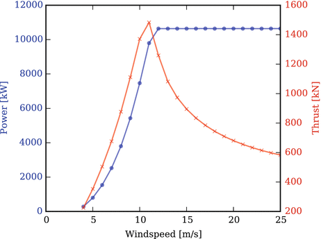
Power and thrust curve of the DTU 10 MW RWT over the operational range
The procedure ensures that the twist is optimal for the reference speed. Away from the reference speed the twist distribution will deteriorate. However, the blade can be pitched to improve the energy yield in those regions. The reference speed for pre-twisting is chosen to maximize annual energy production which depends on the wind speed distribution of the site. A pre-twisting procedure for linear blade deflections is proposed by Lobitz and Veers (2003) and extended to non-linear blade deflections by Stäblein et al. (2016). The latter show that pre-twisting significantly reduces the power loss in annual energy production of the DTU 10 MW RWT.
-
(2)
Optimize the twist, and probably also the chord, distribution of the coupled blade for a given wind speed distribution. The tip-speed ratio might also be considered an optimization variable. To the authors knowledge there has not been a study that pursued this approach.

In the following, the pre-twist procedure presented by Stäblein et al. (2016) is revisited. As a constant coupling coefficient is applied along the length of the blade, the resulting pre-twist distribution provides a good indication of the blade regions where coupling is most efficient.
3.1 Pre-Twisting Procedure
Pre-twisting adjusts the structural twist of a coupled blade in an iterative procedure to provide the same angle of attack along the blade as the uncoupled blade for a given reference wind speed. The first step is to calculate the steady state angle of attack along the uncoupled α ref and coupled blade α btc at the reference wind speed v ref . The angle of attack is chosen as a reference as it results in the same aerodynamic state, irrespective of the blade twist which is not uniquely defined for large displacements and rotations. The difference between the angles of attack Δ α is then imposed on the coupled blade as a pre-twist. Both steps are repeated until the angle of attack along the uncoupled and coupled blade are identical at the reference speed. A flowchart of the procedure is shown in Fig. 5.4. The power curve is further improved by recalculating the optimal pitch angle over the operational range of the turbine. Pre-twisting results in an identical angle of attack along the blade at the reference wind speed v ref . Below the reference speed, the thrust on the blade is lower which results in reduced bending and consequently less coupling induced twist. The blade therefore has a higher angle of attack slope along the blade as the blade twists towards stall. In this region, it is important to consider the angle of attack limit when determining the optimal pitch angle in order to avoid flow separation. Above the reference speed, where thrust is larger, the coupling will result in a lower angle of attack slope along the blade as the blade twists towards feather.

Flowchart of the pre-twisting procedure presented by Stäblein et al. (2016)
3.2 Coupling Distribution
If bend-twist coupling is introduced by utilising the anisotropic properties of the blade material, the change in fibre direction in the spar caps and/or skin of the blade results in a reduced bending stiffness. Previous studies (Fedorov and Berggreen 2014) have shown that coupling reduces the bending stiffness of the blade by 30–35 % when no material is added. As the tower clearance of the blade tip is often a governing design criteria a loss in stiffness is undesirable and it is advisable to introduce the coupling only in blade regions where it is most efficient. Figure 5.5 shows the coupling induced twist and the flapwise curvature at 8 m/s reference speed for the DTU 10 MW RWT with a constant flap-twist to feather coupling coefficient of 0.2 along the blade. It can be seen that the curvature correlates with the slope of the induced twist. The relationship can also be shown by reducing the cross-sectional constitutive relation (5.4) to flapwise moment and torsion. Assuming torsion to be zero, a linear relationship between curvature and twist rate can be established:

Blade flapwise curvature and coupling induced twist at 8 m/s wind speed (Stäblein et al. 2016)
Returning to Fig. 5.5, the curvature-twist relationship shows that, for the DTU 10 MW RWT, coupling is most efficient in the outer half of the blade. A similar observation is also made by Bottasso et al. (2013) who show that partially coupled blades exhibit a similar load alleviation performance as fully coupled blades.
4 Summary
Bend-twist coupling is a proven technique to reduce the fatigue loads of wind turbine blades. If the coupling is introduced by changing the fibre direction of the anisotropic blade material, it is important to account for the effects the material has on the structural response of the blade. Previous research indicates that shear deformations, general warping and the geometric non-linearity from large displacements need to be considered. An analysis framework that includes all those effects, consisting of cross-section analysis, beam element and co-rotational formulation, has been presented in this chapter. When designing bend-twist coupled blades, pre-twisting can be used to reduce the power loss associated with the coupling. To maintain blade stiffness for tower clearance while utilizing the load alleviation potential of coupled blades, the coupling should only be introduced in regions with high curvature as this is where it is most efficient.
References
Bak C, Zahle F, Bitsche R, et al (2013) The DTU 10-MW reference wind turbine. In: DTU orbit - the research information system. Available via Technical University of Denmark. http://orbit.dtu.dk/files/55645274/The_DTU_10MW_Reference_Turbine_Christian_Bak.pdf. Accessed 08 Apr 2016
Bathe KJ, Bolourchi S (1979) Large displacement analysis of three-dimensional beam structures. Int J Numer Methods Eng 14(7):961–986
Battini JM, Pacoste C (2002) Co-rotational beam elements with warping effects in instability problems. Comput Method Appl M 191(17):1755–1789
Bazoune A, Khulief YA, Stephen NG (2003) Shape functions of three-dimensional Timoshenko beam element. J Sound Vib 259(2):473–480
Berdichevskii VL (1979) Variational-asymptotic method of constructing a theory of shells. J Appl Math Mech 43(4):711–736
Borri M, Merlini T (1986) A large displacement formulation for anisotropic beam analysis. Meccanica 21(1):30–37
Bottasso CL, Campagnolo F, Croce A, Tibaldi C (2013) Optimization-based study of bend-twist coupled rotor blades for passive and integrated passive/active load alleviation. Wind Energy 16(8):1149–1166
Capellaro M, Kühn M (2010) Boundaries of bend twist coupling. In: Voutsinas S (ed) Torque 2010: the science of making torque from wind, Crete, 2010
Cardona A, Geradin M (1988) A beam finite element non-linear theory with finite rotations. Int J Numer Methods Eng 26(11):2403–2438
Cesnik CES, Hodges DH (1997) VABS: a new concept for composite rotor blade cross-sectional modeling. J Am Helicopter Soc 42(1):27–38
Chandra R, Chopra I (1992) Structural response of composite beams and blades with elastic couplings. Compos Eng 2(5–7):347–374, wOS:A1992HZ76200006
Cortínez VH, Piovan MT (2002) Vibration and buckling of composite thin-walled beams with shear deformability. J Sound Vib 258(4):701–723
Crisfield MA (1990) A consistent co-rotational formulation for non-linear, three-dimensional, beam-elements. Comput Method Appl M 81(2):131–150
Fedorov V, Berggreen C (2014) Bend-twist coupling potential of wind turbine blades. J Phys Conf Ser 524:012035
Giavotto V, Borri M, Mantegazza P, Ghiringhelli GL, Carmaschi V, Maffioli GC, Mussi F (1983) Anisotropic beam theory and applications. Comput Struct 16(1):403–413
Guyan RJ (1965) Reduction of stiffness and mass matrices. AIAA J 3(2):380–380
Hodges DH (1990a) A mixed variational formulation based on exact intrinsic equations for dynamics of moving beams. Int J Solids Struct 26(11):1253–1273
Hodges DH (1990b) Review of composite rotor blade modeling. AIAA J 28(3):561–565
Jung SN, Nagaraj VT, Chopra I (1999) Assessment of composite rotor blade modeling techniques. J Am Helicopter Soc 44(3):188–205
Kim T, Hansen AM, Branner K (2013) Development of an anisotropic beam finite element for composite wind turbine blades in multibody system. Renew Energ 59:172–183
Lobitz DW, Laino DJ (1999) Load mitigation with twist-coupled HAWT blades. In: ASME/AIAA wind energy symposium, Reno, NV, pp 124–134
Lobitz DW, Veers PS (1998) Aeroelastic behavior of twist-coupled HAWT blades. In: ASME/AIAA wind energy symposium, Reno, NV, pp 75–83
Lobitz DW, Veers PS (2003) Load mitigation with bending/twist-coupled blades on rotors using modern control strategies. Wind Energy 6(2):105–117
Rehfield LW, Atilgan AR, Hodges DH (1990) Nonclassical behavior of thin-walled composite beams with closed cross sections. J Am Helicopter Soc 35(2):42–50
Simo J, Vu-Quoc L (1986) A three-dimensional finite-strain rod model. Part II: computational aspects. Comput Method Appl M 58:79–116
Smith EC, Chopra I (1991) Formulation and evaluation of an analytical model for composite box-beams. J Am Helicopter Soc 36(3):23–35
Stäblein AR, Hansen MH (2016) Timoshenko beam element with anisotropic cross-sectional properties. In: VII European congress on computational methods in applied sciences and engineering (ECCOMAS 2016), Crete Island
Stäblein AR, Tibaldi C, Hansen MH (2016) Using pretwist to reduce power loss of bend-twist coupled blades. In: 34th wind energy symposium, p 1010
Timoshenko SP (1921) On the correction for shear of the differential equation for transverse vibrations of prismatic bars. Philos Mag 41(245):744–746
Verelst DR, Larsen TJ (2010) Load Consequences when sweeping blades - a case study of a 5 MW pitch controlled wind turbine. Tech. Rep. Risø-R-1724(EN), Risø National Laboratory for Sustainable Energy
Volovoi VV, Hodges DH, Cesnik CES, Popescu B (2001) Assessment of beam modeling methods for rotor blade applications. Math Comput Modell 33(10–11):1099–1112
Open Access
This chapter is distributed under the terms of the Creative Commons Attribution-NonCommercial 4.0 International License (http://creativecommons.org/licenses/by-nc/4.0/), which permits any noncommercial use, duplication, adaptation, distribution and reproduction in any medium or format, as long as you give appropriate credit to the original author(s) and the source, provide a link to the Creative Commons license and indicate if changes were made.
The images or other third party material in this chapter are included in the work’s Creative Commons license, unless indicated otherwise in the credit line; if such material is not included in the work’s Creative Commons license and the respective action is not permitted by statutory regulation, users will need to obtain permission from the license holder to duplicate, adapt or reproduce the material.
Author information
Authors and Affiliations
Corresponding author
Editor information
Editors and Affiliations
Rights and permissions
Open Access This chapter is distributed under the terms of the Creative Commons Attribution-NonCommercial 4.0 International License (http://creativecommons.org/licenses/by-nc/4.0/), which permits any noncommercial use, duplication, adaptation, distribution and reproduction in any medium or format, as long as you give appropriate credit to the original author(s) and the source, provide a link to the Creative Commons license and indicate if changes were made.
The images or other third party material in this chapter are included in the work’s Creative Commons license, unless indicated otherwise in the credit line; if such material is not included in the work’s Creative Commons license and the respective action is not permitted by statutory regulation, users will need to obtain permission from the license holder to duplicate, adapt or reproduce the material.
Copyright information
© 2016 The Author(s)
About this chapter
Cite this chapter
Stäblein, A.R. (2016). Analysis and Design of Bend-Twist Coupled Wind Turbine Blades. In: Ostachowicz, W., McGugan, M., Schröder-Hinrichs, JU., Luczak, M. (eds) MARE-WINT. Springer, Cham. https://doi.org/10.1007/978-3-319-39095-6_5
Download citation
DOI: https://doi.org/10.1007/978-3-319-39095-6_5
Published:
Publisher Name: Springer, Cham
Print ISBN: 978-3-319-39094-9
Online ISBN: 978-3-319-39095-6
eBook Packages: EnergyEnergy (R0)