
Abstract
This chapter presents the theoretical basis of the vibration analysis method applied to the field of tie rods. The elements obtained during acquisition are then used to obtain results concerning free and total lengths, the diameters of the elements tested and the dynamic stiffness used to calculate the internal force at the tie-rod.
You have full access to this open access chapter, Download chapter PDF
Radio waves are electromagnetic waves of the same nature as light, which result from the disturbance of electric and magnetic fields.
In addition to visible light, there are radar waves, microwaves, infrared, ultraviolet, X and gamma rays, and radio waves.
Our area of intervention is sound. Of sound waves need material support to spread, electromagnetic waves, spread better in a vacuum, and much faster: sound only goes at 300 m/s, while electromagnetic waves go at about 300,000 km/s. You see lightning before you hear thunder.
1.1 Definitions—Period—Frequency
In addition to visible light, there are radar waves, microwaves, infrared, ultraviolet, X-rays, gamma rays and radio waves. Our operating range is generally below 2000 Hz.
A wave is the modification of the physical state of a physical environment. In our case, it's a reinforcement, usually steel, contained in a cylinder of cement grout. The wave propagates as a result of local action, with a velocity determined by the characteristics of the material through which it passes.
A periodic function is a function which, when applied to a variable, takes on the same value as a certain fixed quantity called period is added to that variable (Fig. 1.1).

Wave / period “T” example
The period T is the time between the passage of two maxima.
Frequency f is a measure of the number of times a periodic phenomenon repeats per unit time f = 1/T (Fig. 1.2).

Sinusoidal waves of different frequencies. − the lower one has the high frequency. − the upper one has the lower one.
The frequency is the number of periods per unit time, which is the inverse of the period: f = 1/T where f is the frequency in Hertz (Fig. 1.3).

Types of frequency
1.2 Principle of the Method
The principle of the method is described in:
-
European Patent Office PCT/FR2005/001597 (Appendix A)
-
WIPO Patent No. WO 2006/010830 A1, 2006 (Appendix B)
The method consists of:
-
Delivering a mechanical shock to the head of the tested element by means of a hammer equipped with a force sensor.
-
Measure the particle velocity at the head of the test item.
-
Do the acquisition in time mode.
-
And analyze the signal in frequency mode.
The figure below visualizes the compression wave emitted by the impact of the hammer and which propagates inside the tested element to go up at its extremity (Fig. 1.4).

Diagram of the compression wave
1.3 Mechanical Impedance
Impedance in a circuit fed by an alternating current is equivalent to resistance.
It is the factor that absorbs the energy used.
Whatever it is:
-
Electrical
-
Mechanical
-
Acoustics
Mechanical impedance is a measure of the resistance to motion of a structure subjected to a given periodic force. It refers to the velocity forces acting on a mechanical system. The mechanical impedance of a point relative to a structure is the relationship between the force applied at a point and the resulting velocity at that point. Mechanical impedance is the inverse of mechanical admittance or mobility.
Example of a curve resulting from a mechanical impedance test:
F in Newton V in m/s V/F in m/sN, frequency in Hz (Figs. 1.5 and 1.6).

V/F curve as a function of frequency

Vibratory responses
The blue test curve (1) is the geometric sum of the three green (3) and two red curves (2 and 4). These curves correspond to different vibration responses of the tested element.
1.4 Ties Rods
A tie rod has
-
A high strength steel bar or strand wire
-
A free part and a sealed part
-
A cement grout to protect the tie rod and ensure the bond with the soil (Figs. 1.7 and 1.8).

Source Rincent BTP—Recife
Cleaning the head and fixing the geophone 3D.

Example: free length and sealed length
Equipment—Force and Velocity (Fig. 1.9).

Source Rincent BTP—France
Hammer with different ends.
The force sensor is piezoelectric.
Piezoelectricity is the property of certain materials to polarize electrically under the action of a mechanical stress and, conversely, to deform when an electric field is applied.
Equipment measures millivolts as a function of time (Fig. 1.10).

Force versus time
Geophone velocity measurement.
The principle of operation of the geophone is that the movement of the support on which it is fixed causes the magnet in the solenoid to move, which creates an electric current linked to the movement. Without movement there is no current measurement (Fig. 1.11).

Source Rincent BTP—France
Geophone, working principle.
For velocity measurement equipment is the geophone 3D or accelerometer (Figs. 1.12, 1.13 and 1.14).

Velocity as a function of time

Realization of the impact. Source Rincent BTP—Recife

Force and velocity as a function of time test results
Changing from temporal mode of acquisition to frequency mode for analysis of results. The Fourier transform is an operation that allows non-periodic signals to be represented in frequency.
The calculation method that allows you to pass in a reversible way from a function to the corresponding trigonometric series is the Fourier transform. This very fruitful method has become a must-have in signal theory, with important applications for the processing and compression of sound and digital images, JPEG image compression, or the 3G and 4G telephony standards are derived directly.
Fourier Transform.
Any curve can be decomposed into a sum of sinusoidal curves of different frequencies with a different weighting coefficient. This operation allows you to switch from time mode to frequency mode (Figs. 1.15 and 1.16).

Fourier transform

Non-periodic curve and sum of periodic functions
Fourier Transform for Velocity (Fig. 1.17).

Fourier transform for velocity
The next step is to establish V/F as a function of frequency (Fig. 1.18).

V/F curve as a function of frequency
After 2000 Hz the force function of frequency is close to zero. V/F curve shows two parts one before 2000 Hz and one after 2000 Hz (Fig. 1.19).

V/F curve function of frequency filtered curve
Time x Frequency
A short phenomenon in time covers wide frequency ranges. In the case of thunderstorms and lightning, the electrical discharge is a short phenomenon that emits over a wide frequency range, causing disruption to radio and TV signals.
For an earthquake the phenomenon is long in a limited frequency range of 2 to 4 Hz.
A hammer with a metal end will produce in a frequency range of 0 to 5000 Hz, and with a “matte” impact elastomer end from 0 to 2000 Hz.
For us, the latter option we used.
Evaluating the V/F curve as a function of frequency
The first step is to calculate the length of the tested element (Fig. 1.20).

Calculating tie rod length
The value of the plane wave propagation velocity in concrete for calculation is 4000 m/s. This theoretical value is given by the testing standard.
There can be two vibration responses that will correspond to the total part of the tie and the part of soils with low mechanical characteristics found in the first meters of the tie (Fig. 1.21).

Two vibration regimes
Example of the tie rod: Free part and total length of the tie rod (Figs. 1.22 and 1.23).

Tie rod, free part and total tie rod

Analyzing test results
Overall length:
-
23,1m with a velocity assumption of 3500m/s
-
26,0m with a velocity assumption of 4000m/s (Fig. 1.24)
Fig. 1.24 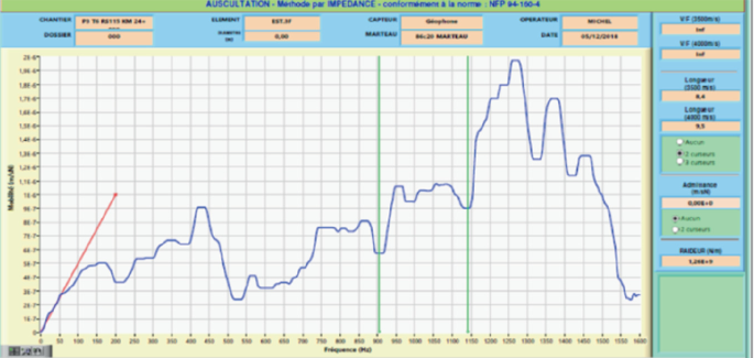
Same test, second vibration regime

Length free part:
-
8.4m with a velocity assumption of 3500m/s
-
9.5m with a velocity assumption of 4000m/s
Mobility.
The mobility read directly on the y-axis allows you to calculate the diameter of the tested element (Fig. 1.25).

Mobility as a function of diameter of the tested element
V/F = 1 / ρb V b A
Concrete volume mass ρb in kg/m3
Circular cross section (m2)
Dynamic stiffness (Fig. 1.26).

Dynamic stiffness calculation
Dynamic stiffness equals 2πb/a and is a complex number.
A complex number is of the type z = x + iy, X is real, Y is imaginary (Fig. 1.27).

Source Rincent BTP—France
Simultaneous static and dynamic testing.
Simultaneous static testing and non-destructive testing allow the following figure to be drawn (Figs. 1.28 and 1.29).

Dynamic strength and stiffness

Example of a stiffness versus force curve (Tons)
Real and imaginary part of stiffness.
A thesis “Measurements and Modelling of Resilient Rubber Rail-pads” by Klaus Knothe, MinyiYu, Mrs. HeikeIlias shows that stiffness part real and part imaginary is constant before 80 Hz (Fig. 1.30).

Dynamic stiffness real part and imaginary part
Static stiffness.
Static stiffness of an element under a load is the slope of the calculated curve under this load (Fig. 1.31).

Static stiffness under 3000 kN load
Philippe Guillermain's thesis shows that there is a direct link between dynamic stiffness and static stiffness, dynamic stiffness is higher than static stiffness, there is a constant relationship between the two stiffnesses for an identical situation.
Stiffness has the same units as modulus.
The Rd/Rs calculations were done from tests on tie rods, the relationship between dynamic and static stiffness and 31 by following example (Fig. 1.32).

Rd/Rs for different loads (tons)
This rule can be checked for other elements, e.g., micro piles in tension (Fig. 1.33).

Rd/Rs for different loads (kN)
Author information
Authors and Affiliations
Corresponding author
Rights and permissions
Open Access This chapter is licensed under the terms of the Creative Commons Attribution 4.0 International License (http://creativecommons.org/licenses/by/4.0/), which permits use, sharing, adaptation, distribution and reproduction in any medium or format, as long as you give appropriate credit to the original author(s) and the source, provide a link to the Creative Commons license and indicate if changes were made.
The images or other third party material in this chapter are included in the chapter's Creative Commons license, unless indicated otherwise in a credit line to the material. If material is not included in the chapter's Creative Commons license and your intended use is not permitted by statutory regulation or exceeds the permitted use, you will need to obtain permission directly from the copyright holder.
Copyright information
© 2024 The Author(s)
About this chapter

Cite this chapter
Rincent, JJ.H. (2024). Waves-Vibratory Analysis. In: Ground Anchors. Springer, Singapore. https://doi.org/10.1007/978-981-97-4414-5_1
Download citation
DOI: https://doi.org/10.1007/978-981-97-4414-5_1
Published:
Publisher Name: Springer, Singapore
Print ISBN: 978-981-97-4413-8
Online ISBN: 978-981-97-4414-5
eBook Packages: EngineeringEngineering (R0)