
Abstract
Based on the effects of white noise and colored noise, we propose a stochastic Holling-III predator–prey model in an impulsive polluted environment. Firstly, we prove an existence and uniqueness theorem of the presented model. Secondly, we establish sufficient criteria of extinction, nonpersistence in mean, and weak persistence in mean for both prey and predator species. Thirdly, with the aid of Lyapunov functions, we prove that this system is ergodic and has a unique stationary distribution under certain conditions. Finally, we verify the theoretical results by performing some numerical simulations.
1 Introduction
Environmental pollution from various industries attracts more and more demographers and ecologists because it has seriously threatened the survival of humans and other exposed living organisms [2, 26, 38]. In the early years, the survival analysis of populations in the polluted environment was carried out by establishing deterministic models. For example, Hallam et al. [3, 6–8] used some deterministic models to show the effects of toxicant on populations, He and Wang [10, 11] analyzed the dynamics of two single-species models in polluted environments, and so on.
The deterministic models are not suitable for modeling the ubiquitous noise-driven systems, so stochastic models in the polluted environment are frequently used to explore the dynamics behavior of species [27]. Generally, there are two main types of environmental noise, white noise and colored noise. For white noise-driven models, Gard [5] investigated a stochastic single-species model to explain the influence of the toxicant on organisms and compared it to the corresponding deterministic model. Liu and Wang [20] studied the dynamics of stochastic single-species population models with and without pollution. Wei et al. [36, 37] further investigated the stochastic single-species population model in a polluted environment. In addition, Lv et al. [23] introduced a new impulsive stochastic chemostat model. On the other hand, to illustrate the switching between two or more environmental regimes, it is meaningful to consider the influence of colored noise on the population [4, 32]. Liu and Wang [21] proposed a stochastic single-specie model under regime switching. Moreover, a stochastic two-species model is presented in [44]. For the dynamics behaviors of the populations with environmental toxins and noises, we also refer the readers to [22, 34, 39, 43] and references therein.
Many models mentioned are based on the Lotka–Volterra model with linear functional responses. However, these models ignore some important natural phenomena (compared with the models with nonlinear functional responses), especially for the predator–prey case [9, 28]. To this end, Holling [12, 13] proposed the most widely used functional responses and classified them into three basic types (denoted types I, II, and III). As a typical nonlinear functional response, Holling type III [29] has a powerful role in describing the predation behavior of vertebrates, for example, some predators learn more special skills for hunting or prey handling. Recently, some important models with Holling type III has been discussed. For instance, Huang et al. [14] established a prey–predator model with Holling-III response function and a prey refuge to show that the refuge has a steadying influence on prey–predator interactions. Su et al. [33] indicated that both periodically varying environment and stochastically released natural enemies have a great impact on the survival of the species by using the predator–prey system with generalized Holling-III type functional response. Wu and Li [40] combined Holling-III type with Hassell–Varley type functional responses to demonstrate the permanence and global attractivity of a discrete predator–prey system. More recently, Sengupta et al. [30] analyzed the dynamics of the deterministic and stochastic models with Holling-III response function, respectively.
To the best of our knowledge, there are rare results on the effects of pollution inputs and noise fluctuations for the dynamics behavior of Holling-III predator–prey systems. Undoubtedly, the theoretical analysis of Holling type-III is more challenging than other functional responses because its nonlinear form is more complicated. In this paper, we are devoted to two main goals:
-
to analyze the long-time behavior of stochastic Holling-III predator–prey systems with regime switching in an impulsive polluted environment, and
-
to investigate the effects of pollution inputs and noise fluctuations on the dynamics of predators and preys.
In particular, when the considered model of this paper reduces to that of [30], our conditions in Theorem 3.2 are more convenient to verify the weak persistence in the mean of predator species in comparison with [30, Theorem 4.4].
This paper is organized as follows. In Sect. 2, we begin to state our model and prepare some preliminaries including the existence of a unique positive solution. In Sect. 3, we obtain some sufficient conditions of the extinction and weak persistence in mean for two species. In Sect. 4, we investigate the existence and uniqueness of stationary distribution. In Sect. 5, we present numerical simulations confirming our theoretical results. Finally, in the last section, we give a brief conclusion.
2 The model and preliminaries
We begin this section by stating the stochastic Holling-III predator–prey model with Markovian switching in an impulsive polluted environment step by step and prepare some preliminaries including the existence and uniqueness theorem.
2.1 The model
First, let us introduce the deterministic Holling-III predator–prey model [41]
with the initial value \((x(0),y(0)) \in \mathbb{R}_{+}^{2}\), where \(x(t)\) and \(y(t)\) denote the population densities of prey and predator species at time t, respectively, \(a_{1}\) and \(a_{2}\) stand for the intrinsic growth rate of prey population and the death rate of predator population, respectively. Both \(b_{1}\) and \(b_{2}\) represent intraspecific coefficients of competition. The nonlinear function \(\frac{\alpha x^{2}}{1+\beta x^{2}}\) is the Holling-III functional response, where α stands for the predation rate of predators on prey populations, β denotes the handling time of predators for each prey that is consumed, and k denotes the conversion rate concerning the number of newborn predators for each captured prey. All parameters of the model are positive.
Taking into account the impact of environmental pollution on species [3, 6–8], most of the existing studies assume that the exogenous input of toxicant is continuous. However, the actual situation is that the toxin is released in regular pulses; for example, the factories drain sewage into rivers on a regular basis. Therefore we focus on the case of toxic exogenous pulse input and then obtain the following model:
where \(\bigtriangleup \chi (t) = \chi (t^{+}) - \chi (t)\) with \(\chi = x,y,C_{1},C_{2},C_{E}\), \(C_{1}(t)\), \(C_{2}(t)\), and \(C_{E}(t)\) stand for the concentrations of toxicant in the organism of the prey, predator, and environment at time t, respectively, \(r_{1}\) and \(r_{2}\) denote the dose-response of the prey and predator to the toxicant, respectively, \(e_{i}\) is the uptake rate of toxicant from environment, \(g_{i}\) and \(m_{i}\) indicate the excretion and depuration rates of toxicant, respectively, h is the loss rate of toxicant, and u and ρ represent the toxicant input amount and the period of the exogenous toxicant input, respectively. Here we assume that the environmental capacity is large enough so that the effects of toxins excreted by the organism into the environment have negligible influences on the concentration of environmental toxins.
Now we further take the white noise into consideration. Following the approach used in [15, 17, 19], the parameters \(a_{1}\) and \(-a_{2}\) of system (2.2) are perturbed with
where the dot denotes the time formal derivative, \(B_{1}(t)\) and \(B_{2}(t)\) are mutually independent one-dimensional standard Brownian motions defined on the complete probability space \((\Omega,\mathcal{F},\{\mathcal{F}_{t}\}_{t\geq 0},\mathbb{P})\), and \(\sigma _{i}^{2}\ (i = 1, 2)\) are the intensities of the white noises. Thus system (2.2) becomes the stochastic Holling-III predator–prey model in the impulsive polluted environment
It is worth pointing out that there are many phenomena that cannot be modeled by Brownian motion-driven stochastic differential equations (SDEs) [45]; for example, when the growth environment of some species changes significantly, their birth and death rates will be much different [1, 46]. In general, the switching among different environments is memoryless, and the waiting time of the next switch obeys an exponential distribution. Hence these random changes can be described by a continuous-time Markov chain \(\xi (t)\), \(t>0\), taking values in a finite-state space \(\mathbb{S}=\{1, 2, \ldots,N\}\) with the generator \(\Gamma =(\gamma _{ij})_{N\times N}\) given by
where \(\gamma _{ij}>0\) is the transition rate from state i to state j if \(i\neq j\), and \(\gamma _{ii}=-\sum_{j\neq i}\gamma _{ij}\). Finally, model (2.3) can be formulated as
where all functions \(a_{i}, b_{i}, r_{i}, \sigma _{i}\ (i=1, 2)\) and \(\alpha, \beta, k\) are \(\mathbb{R}_{+}\)-valued. In addition, we assume that \(\xi (t)\) is irreducible and independent of Brownian motions \(B_{i}(t)\ (i=1,2)\). In fact, the Markov chain \(\xi (t)\) has a unique stationary distribution \(\pi =(\pi _{1}, \pi _{2},\ldots,\pi _{N})\in \mathbb{R}^{1\times N}\), which can be obtained by solving the linear equation \(\pi \Gamma =0\) subject to \(\sum^{N}_{j=1}\pi _{j}=1\) and \(\pi _{j}>0, j\in \mathbb{S}\). As a result, for any vector \(\theta =(\theta (1), \ldots, \theta (N))^{T}\), \(\lim_{t\rightarrow \infty }\frac{1}{t}\int ^{t}_{0}\theta (\xi (s)) \,\mathrm{d}s=\sum_{i\in \mathbb{S}}\pi _{i}\theta (i)\). In reality, environmental noise has little effect on the toxin concentration of the organism, so we assume that the parameters \(e_{i}\), \(g_{i}\), \(m_{i}\), and h are independent of noises.
2.2 Preliminaries
For convenience, define \(f^{*}=\limsup_{t\rightarrow \infty }f(t),\ f_{*}=\liminf_{t\rightarrow \infty }f(t)\), \(\langle f\rangle = \frac{1}{t} \int ^{t}_{0}f(s) \,\mathrm{d}s\), \(\check{g}=\max_{i\in \mathbb{S}}g(i)\), and \(\hat{g}=\min_{i\in \mathbb{S}}g(i)\). For the subsystem of model (2.4),
with initial values \(C_{i}(0)\in (0,1)\ (i=1, 2)\) and \(C_{E}(0)\in (0,1)\), the following lemma is taken from [18].
Lemma 2.1
For subsystem (2.5), we have:
-
(1)
it admits a unique positive ρ-periodic solution \((\overline{C}_{1}(t), \overline{C}_{2}(t), \overline{C}_{E}(t))^{T}\);
-
(2)
for any \(\varepsilon >0\) and sufficiently large t,
$$\begin{aligned} \overline{C}_{i}(t)-\varepsilon < C_{i}(t)< \overline{C}_{i}(t)+ \varepsilon,\quad i=1, 2; \end{aligned}$$(2.6) -
(3)
and
$$\begin{aligned} \lim_{t\rightarrow \infty } \frac{1}{t} \int _{0}^{t} C_{i}(s) \,\mathrm{d}s = \lim_{t\rightarrow \infty } \frac{1}{t} \int _{0}^{t} \overline{C}_{i}(s) \, \mathrm{d}s = \frac{e_{i}u}{h(g_{i}+m_{i})\rho } =: \frac{G_{i}}{\rho },\quad i=1, 2. \end{aligned}$$(2.7)
Because \(C_{1}(t)\), \(C_{2}(t)\), and \(C_{E}(t)\) can be obtained only from (2.5), system (2.4) reduces to the subsystem
with initial values
Subsystem (2.8) can be written as the SDE
with initial value \((z(0),\xi (0)) = (z_{0},\xi _{0})\), where the drift coefficient \(f: \mathbb{R}^{n}\times \mathbb{S}\rightarrow \mathbb{R}^{n}\), the diffusion coefficient \(g: \mathbb{R}^{n}\times \mathbb{S}\rightarrow \mathbb{R}^{n\times d}\), and \(B(t)\) is a d-dimensional Brownian motion. Let \(D(z, k)=g(z, k)g(z, k)^{T}=(d_{ij}(z, k))\). For a a twice continuously differentiable function \(V(z, k): \mathbb{R}^{n}\times \mathbb{S}\rightarrow \mathbb{R}\), we define the diffusion operator \(\mathcal{L}\) by
We end this section with the following existence and uniqueness theorem.
Theorem 2.1
For any given initial value \((x(0), y(0), \xi (0))\in \mathbb{R}^{2}_{+}\times \mathbb{S}\), there exists a unique global solution to system (2.8), and \((x(t), y(t), \xi (t))\in \mathbb{R}^{2}_{+}\times \mathbb{S}\) a.s.
Proof
Since both the drift and diffusion coefficients of equation (2.8) satisfy the local Lipschitz condition, there is a unique local solution \((x(t), y(t), \xi (t))\) on \(t\in [0, \tau _{e})\), where \(\tau _{e}\) denotes the explosion time (see [25]). To verify that the solution is global, we need to prove that \(\tau _{e}=\infty \) a.s. Let \(m_{0}>1\) be sufficiently large such that \(x(0), y(0) \in [1/m_{0}, m_{0}]\). For each integer \(m\geq m_{0}\), define the stopping time
with convention \(\inf \emptyset =+\infty \). It is clear that \(\tau _{m}\) increases as \(m\rightarrow \infty \). Let \(\tau _{\infty }=\lim_{m\rightarrow \infty }\tau _{m}\), so that \(\tau _{\infty }\leq \tau _{e}\). Thus we only need to prove that \(\tau _{\infty }=\infty \) a.s. If this were not true, then there would be constants \(T>0\) and \(\epsilon \in (0,1)\) such that \(\mathbb{P}\{\tau _{\infty }\leq T\}>\epsilon \) and an integer \(m_{1}\geq m_{0}\) such that
Define the \(C^{2}\)-function V: \(\mathbb{R}_{+}^{2}\times \mathbb{S}\rightarrow \mathbb{R}_{+}\) as follows:
According to the definition of the operator \(\mathcal{L}\) (see (2.11)) and the vertex formula of quadratic functions, we have
where H is a finite positive constant. Then the generalized Itô’s formula [25] yields
which implies
where \(\tau _{m}\wedge T = \min \{\tau _{m}, T\}\). On the other hand, set \(\Omega _{m}=\{\tau _{m}\leq T \}\) for \(m\geq m_{1}\), so \(\mathbb{P}(\Omega _{m})\geq \epsilon \) by (2.12). Note that for all \(\omega \in \Omega _{m}\), at least one of \(x(\tau _{m},\omega )\) and \(y(\tau _{m},\omega )\) equals either m or \(1/m\). Then
Reviewing (2.13), we can claim that
where \(1_{\Omega _{m}}\) is the indicator function of the set \(\Omega _{m}\). Letting \(m\rightarrow \infty \) leads to
a contradiction, so that \(\tau _{\infty }=\infty \) a.s. The proof is complete. □
Remark 2.1
By the existence and uniqueness theorem it follows from [42, Lemma 1] that the solution \((x(t), y(t), \xi (t))\) of (2.8) satisfies
3 Extinction and persistence
This section aims to investigate the extinction, nonpersistence in mean, and weak persistence in mean of both prey \(x(t)\) and predator \(y(t)\) separately.
Definition 3.1
The population \(z(t)\) is called:
-
(1)
extinct if \(\lim_{t\rightarrow \infty }z(t)=0\) a.s.;
-
(2)
nonpersistent in mean if \(\limsup_{t\rightarrow \infty } \frac{1}{t}\int _{0}^{t} z(s) \,\mathrm{d}s= 0\) a.s.; and
-
(3)
weakly persistent in mean if \(\limsup_{t\rightarrow \infty } \frac{1}{t}\int _{0}^{t} z(s) \,\mathrm{d}s > 0\) a.s.
For convenience, we define
Theorem 3.1
The prey \(x(t)\) of (2.8) is
-
(1)
extinct if \(A_{1}- B_{1}<0\);
-
(2)
nonpersistent in mean if \(A_{1}- B_{1}=0\); and
-
(3)
weakly persistent in mean if \(A_{1}- B_{1}>0\).
Proof
Applying generalized Itô’s formula to (2.8) yields
where \(M_{i}(t)=\int ^{t}_{0}\sigma _{i}(\xi (s)) \,\mathrm{d}B_{i}(s)\ (i=1,2)\) satisfy (see [24, Theorem 3.4])
Firstly, it follows from equation (3.1) that
Using (3.3) and the ergodicity of \(\xi (t)\), we obtain
which implies that \(\lim_{t\rightarrow \infty }x(t)=0\) a.s., so the prey \(x(t)\) is extinct, and (1) is proved.
Secondly, for given \(\epsilon > 0\) small, there exists a constant \(\widetilde{T}>0\) such that for all \(t>\widetilde{T}\),
Inserting (3.5) into (3.1) leads to
By [19, Lemma 2], if \(A_{1}-B_{1}\geq 0\), then
In particular, when \(A_{1}-B_{1}=0\), it follows from (3.6) and the arbitrariness of ϵ that \(\langle x(t) \rangle ^{*} = 0\) a.s., which states that the prey \(x(t)\) is nonpersistent in mean. So (2) is proved.
Thirdly, taking the upper limits of both sides of (3.1) shows
Recalling that \(x(t)^{*} < \infty \) a.s. (see Remark 2.1), we get that the left side of (3.7) is nonpositive. Then
which shows that \(\langle x(t)\rangle ^{*} > 0\). Otherwise, for all \(\omega \in \{\omega: \langle x(t,\omega )\rangle ^{*} =0 \}\), estimate (3.8) gives \(\langle y(t)\rangle ^{*} > 0\). However, since \(\frac{k(\xi )\alpha (\xi )x^{2}}{1+\beta (\xi )x^{2}} \leq \frac{\check{k} \check{\alpha } x}{2\hat{\beta }^{1/2}}, x \in \mathbb{R}_{+}\), another equation (3.2) yields
which shows that \(\langle y(t)\rangle ^{*} = 0\), a contradiction, so \(\langle x(t)\rangle ^{*} >0\) a.s., that is, the prey \(x(t)\) is weakly persistent in mean. Hereto, all conclusions of the theorem are proved. □
Theorem 3.2
The predator \(y(t)\) of (2.8) is
-
(1)
extinct if \(A_{2}- B_{2}<0\);
-
(2)
nonpersistent in mean if \(A_{2}- B_{2}=0\); and
-
(3)
weakly persistent in mean if there exists a constant \(\delta \in (0, \frac{\hat{b}_{1}}{\check{\beta }})\) such that \(A_{3}>0\).
Proof
Firstly, using equation (3.2), we have
Analogously, taking the upper limits on both sides of (3.9) yields
which implies that \(\lim_{t\rightarrow \infty }y(t)=0\) a.s., and thus (1) is proved.
Secondly, for given \(\epsilon > 0\) small, there exists a constant \(\widetilde{T}>0\) such that for all \(t>\widetilde{T}\),
Inserting (3.10) into (3.2), we arrive at
If \(A_{2}-B_{2}\geq 0\), then
In particular, if \(A_{2}-B_{2}=0\), then follows from (3.11) and the arbitrariness of ϵ that \(\langle y(t)\rangle ^{*} = 0\) a.s., and thus (2) is proved.
Finally, by (3.1), (3.2), and the first equation of (2.8) we get
Applying the reverse Young inequality
we get \(\frac{k \alpha x^{2}}{1 + \beta x^{2}} \geq 2\sqrt{\delta k \alpha }x - \delta (1 + \beta x^{2}), x \in \mathbb{R}_{+}\). Then, using the inequality \(-\frac{\alpha x}{1 + \beta x^{2}}y \geq - \frac{(1+\beta )\alpha }{2\beta }y, x,y \in \mathbb{R}_{+}\), we derive that
where we used the vertex formula of quadratic functions. On the other hand, Remark 2.1 reads
Thus \(\langle y(t)\rangle ^{*} > 0\) a.s. Hereto, all conclusions of this theorem are proved. □
Remark 3.1
According to Theorems 3.1 and 3.2, we can observe that
-
(1)
the greater the values of \(\sigma _{i}\ (i=1,2)\), the greater the risk of extinction of \(x(t)\) and \(y(t)\); see Figs. 1 and 2(a);
Figure 1 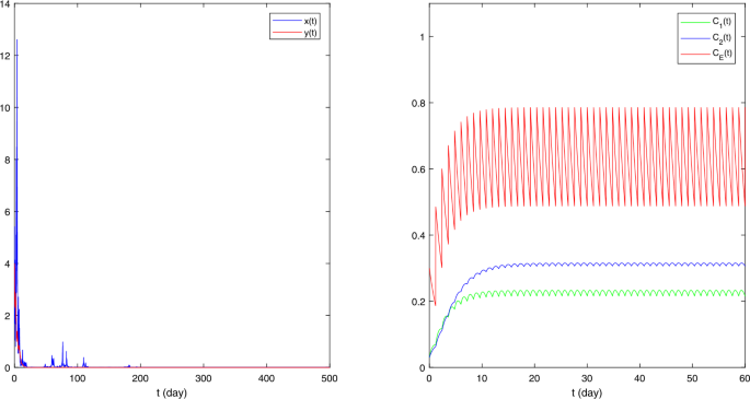
The sample paths of stochastic model (5.1) with \(\pi = (0.9,0.1)\), \(a_{1} = (0.62,0.8)\), \(b_{1} = (0.021,0.04)\), \(\alpha = 0.2\), \(\beta = 0.1\), \(r_{1} = 0.9\), \(\sigma _{1} = 1\), \(a_{2} = (0.2,0.4)\), \(b_{2} = 0.04\), \(k = 0.2\), \(r_{2} = 0.8\), \(\sigma _{2} = 0.2\), \(\rho = 1.2\), \(x_{0} = 5\), \(y_{0} = 4\)
Figure 2 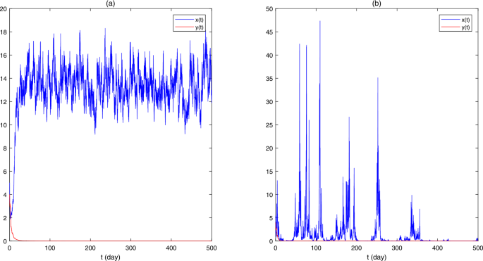
The sample paths of stochastic model (5.1), where (a) \(\pi = (0.9,0.1)\), \(a_{1} = (0.62,0.8)\), \(b_{1} = (0.021,0.04)\), \(\alpha = 0.2\), \(\beta = 0.1\), \(r_{1} = 0.9\), \(\sigma _{1} = 0.1\), \(a_{2} = (0.2,0.4)\), \(b_{2} = 0.04\), \(k = 0.2\), \(r_{2} = 0.8\), \(\sigma _{2} = 0.1\), \(\rho = 1.2\), \(x_{0} = 5\), \(y_{0} = 4\); (b) \(\pi = (0.1,0.9)\), \(a_{1} = (0.62,0.8)\), \(b_{1} = (0.021,0.04)\), \(\alpha = 0.2\), \(\beta = 0.1\), \(r_{1} = 0.9\), \(\sigma _{1} = 1\), \(a_{2} = (0.2,0.4)\), \(b_{2} = 0.04\), \(k = 0.2\), \(r_{2} = 0.8\), \(\sigma _{2} = 0.2\), \(\rho = 1.2\), \(x_{0} = 5\), \(y_{0} = 4\)
-
(2)
the distribution π of Markov chain \(\xi (t)\) plays a significant role in the survival of \(x(t)\) and \(y(t)\); see Figs. 1 and 2(b);
-
(3)
the smaller the value of the impulsive input period ρ, the greater the risk of extinction \(x(t)\) and \(y(t)\); see Figs. 1 and 3.
Figure 3 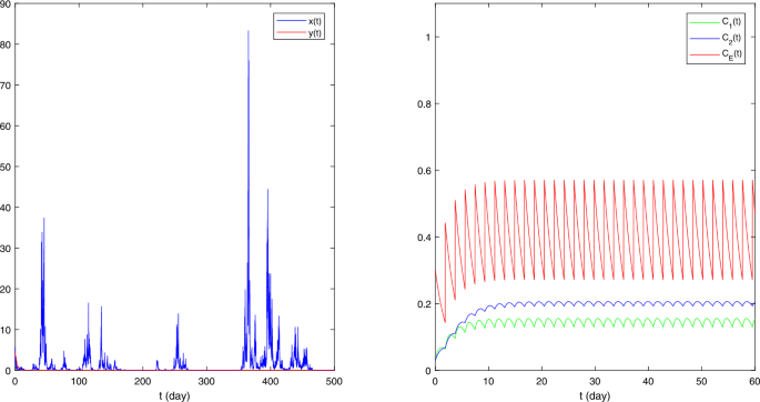
The sample paths of stochastic model (5.1) with \(\pi = (0.9,0.1)\), \(a_{1} = (0.62,0.8)\), \(b_{1} = (0.021,0.04)\), \(\alpha = 0.2\), \(\beta = 0.1\), \(r_{1} = 0.9\), \(\sigma _{1} = 1\), \(a_{2} = (0.2,0.4)\), \(b_{2} = 0.04\), \(k = 0.2\), \(r_{2} = 0.8\), \(\sigma _{2} = 0.2\), \(\rho = 1.86\), \(x_{0} = 5\), \(y_{0} = 4\)


Remark 3.2
When model (2.4) of this paper reduces to [30, model (5)], compared with [30, Theorem 4.4(3)], Theorem 3.2(3) is more convenient to verify the weak persistence in the mean of predator species \(y(t)\), because the conditions of Theorem 3.2(3) are only related to the parameters of equation (2.4).
4 Stationary distribution
In this section, we prove that the solution of model (2.8) has a unique stationary distribution under certain conditions. To facilitate its proof, we will first prove a useful lemma.
Lemma 4.1
Suppose that all of the following conditions hold:
-
(1)
\(\gamma _{ij}>0\) for all \(i\neq j\);
-
(2)
For all \(k\in \mathbb{S}\), the symmetric \(D(\cdot, k)\) admits a constant \(\varrho \in (0, 1]\) such that
$$ \varrho \vert \zeta \vert ^{2}\leq \zeta ^{T}D(z, k) \zeta \leq \varrho ^{-1} \vert \zeta \vert ^{2}, \quad\zeta, z \in \mathbb{R}^{n}; $$ -
(3)
There exists a bounded open set \(\mathcal{D}\subset \mathbb{R}^{n}\) with a regular boundary satisfying that for all \(k\in \mathbb{S}\), there exists a twice continuously differentiable function \(V(\cdot, k): \mathcal{D}^{c}\rightarrow \mathbb{R}_{+}\) such that for some \(\varsigma >0\),
$$\begin{aligned} \mathcal{L}V(z, k)\leq -\varsigma,\quad (z, k)\in \mathcal{D}^{c} \times \mathbb{S}. \end{aligned}$$
Then the solution \((z(t),\xi (t))\) of (2.10) is ergodic and positive recurrent, that is, it has a unique stationary distribution.
Theorem 4.1
If there exists a constant \(\delta \in (0, \frac{\hat{b}_{1}}{\check{\beta }})\) such that \(\lambda:=\sum_{i=1}^{N}\pi _{i}\Phi _{i}>0\), where \(\Phi _{i} = a_{1}(i) - r_{1}(i)(\overline{C}_{1}(t))^{*} -a_{2}(i) -r_{2}(i)( \overline{C}_{2}(t))^{*} - \frac{1}{2}(\sigma _{1}^{2}(i)+\sigma _{2}^{2}(i)) - \delta - \frac{(b_{1}(i)+a_{1}(i)-2\sqrt{\delta k(i)\alpha (i)})^{2}}{4(b_{1}(i)- \delta \beta (i))} -\frac{(b_{2}(i)-a_{2}(i))^{2}}{4b_{2}(i)}\), then the solution \((x(t), y(t), \xi (t))\) of model (2.8) is ergodic and has a unique stationary distribution in \(\mathbb{R}^{2}_{+}\times \mathbb{S}\).
Proof
To use Lemma 4.1, we need to verify its three conditions. The first two conditions of Lemma 4.1 can be easily verified by the same proof of [31], so we omit it. Thus we mainly verify condition (3) of Lemma 4.1. For simplicity, define the \(C^{2}\)-function \(U: \mathbb{R}_{+}^{2} \rightarrow \mathbb{R}\) as
where \(M=\frac{2}{\lambda }\max \{2,\sup_{(x,y)\in \mathbb{R}^{2}_{+}} \{ -\frac{d_{1}}{2}x^{3}+d_{2}x^{2}-\frac{d_{3}}{2}y^{3}+ \frac{d_{4}}{2}y^{2}\} \}>0\), and the positive constants \(d_{i}\ (i = 1,2,3,4)\) will be fixed later. Based on the fact that \(U(x,y)\) has a unique minimum point \(U(x^{*},y^{*})\), we proceed to define the Lyapunov function \(V:\mathbb{R}_{+}^{2}\times \mathbb{S}\rightarrow \mathbb{R}_{+}\) as
where \(\omega =(\omega _{1}, \omega _{1}, \ldots, \omega _{N})\), \(|\omega |=( \omega _{1}^{2} + \omega _{2}^{2} + \cdots + \omega _{N}^{2} )^{1/2}\) with \(\omega _{i}\ (i\in \mathbb{S})\) to determined later. For sufficiently large t, taking into account (2.6) and using generalized Itô’s formula, together with the facts \(\frac{\alpha }{1+\beta x^{2}} xy \leq \alpha xy\), \(-\frac{k\alpha x^{2}}{1+\beta x^{2}} \leq -2\sqrt{\delta k \alpha }x + \delta (1+\beta x^{2})\), \(\frac{k \alpha x^{2}}{1 + \beta x^{2}}y \leq \frac{k \alpha }{2 \beta ^{1/2}}xy\) for all \(\delta,x,y \in \mathbb{R}_{+}\), as well as the vertex formula of quadratic functions, we have
where
Using generalized Itô’s formula again, we have
and
On the other hand, we can observe that
where \(\Phi =(\Phi _{1},\Phi _{2},\ldots,\Phi _{N})^{T}\) and \(\mathbb{I}_{N}=(1,1,\ldots,1)^{T}\in R^{N}\). Since Φ is irreducible, there exists a solution \(\omega =(\omega _{1},\omega _{2},\ldots,\omega _{N})^{T}\) to the following equation (see [16, Lemma 2.3]):
which implies that
Now, combining (4.1)–(4.4), we arrives at
where \(d_{1}=\check{k}^{2}\hat{b}_{1}\), \(d_{2}=\check{k}^{2}( \check{a}_{1} + \frac{1}{2}\check{\sigma }^{2}_{1} )\), \(d_{3}=\hat{b}_{2}\), \(d_{4} = \frac{1}{2}\check{\sigma }^{2}_{2}\), and \(d_{5}=M( \check{\alpha } + \frac{\check{k} \check{\alpha }}{2 \hat{\beta }^{1/2}} ) + \check{k} \check{a}_{1}\). To verify condition (3) of Lemma 4.1, we consider the bounded closed subset
where ε is sufficiently small such that
where
Finally, it remains to prove
where the complement \(\mathcal{D}^{c}_{\varepsilon }\) can be split as \(\mathcal{D}^{c}_{\varepsilon } = \mathcal{D}_{\varepsilon }^{1} \cup \mathcal{D}_{\varepsilon }^{2} \cup \mathcal{D}_{\varepsilon }^{3} \cup \mathcal{D}_{\varepsilon }^{4}\) with
Case 1: \((x,y,i)\in \mathcal{D}_{\varepsilon }^{1}\times \mathbb{S}\). It follows from the estimate \(xy\leq \varepsilon y\leq \varepsilon (1+y^{3})\), the definition of M, and (4.5) that
Case 2: \((x,y,i)\in \mathcal{D}_{\varepsilon }^{2}\times \mathbb{S}\). Since \(xy\leq \varepsilon x\leq \varepsilon (1+x^{3})\), we also have
Case 3: \((x,y,i)\in \mathcal{D}_{\varepsilon }^{3}\times \mathbb{S}\). Based on (4.6), we have
Case 4: \((x,y,i)\in \mathcal{D}_{\varepsilon }^{4}\times \mathbb{S}\). Similarly,
To summarize, condition (3) of Lemma 4.1 is satisfied. Therefore we obtain the desired assertion. □
5 Numerical simulations
In this section, we perform some numerical simulations to verify the theoretical results established in the previous sections.
Example 5.1
Consider the following stochastic Holling-III predator–prey model with Markovian switching in an impulsive polluted environment:
with the initial value \((x(0), y(0), C_{1}(0), C_{2}(0), C_{E}(0)) = (x_{0},y_{0},0.03,0.03,0.3)\), where \(\xi (t)\) is a Markov chain with \(\xi (0) = 1\) and state space \(\mathbb{S} = \{1,2\}\).
(i) In Fig. 1, we take \(\pi = (0.9,0.1)\), \(a_{1} = (0.62,0.8)\), \(b_{1} = (0.021,0.04)\), \(\alpha = 0.2\), \(\beta = 0.1\), \(r_{1} = 0.9\), \(\sigma _{1} = 1\), \(a_{2} = (0.2,0.4)\), \(b_{2} = 0.04\), \(k = 0.2\), \(r_{2} = 0.8\), \(\sigma _{2} = 0.2\), \(\rho = 1.2\), \(x_{0} = 5\), \(y_{0} = 4\). By simple calculation, \(A_{1} - B_{1} = -183/2750 < 0\) and \(A_{2} - B_{2} = -9/100 < 0\). Theorems 3.1 and 3.2 indicate that both \(x(t)\) and \(y(t)\) will go to extinction. Figure 1 is consistent with the result.
(ii) In Fig. 2(a), we take \(\pi = (0.9,0.1)\), \(a_{1} = (0.62,0.8)\), \(b_{1} = (0.021,0.04)\), \(\alpha = 0.2\), \(\beta = 0.1\), \(r_{1} = 0.9\), \(\sigma _{1} = 0.1\), \(a_{2} = (0.2,0.4)\), \(b_{2} = 0.04\), \(k = 0.2\), \(r_{2} = 0.8\), \(\sigma _{2} = 0.1\), \(\rho = 1.2\), \(x_{0} = 5\), \(y_{0} = 4\). The only difference between the parameters of Figs. 1 and 2(a) is the noise intensities \(\sigma _{1}\) and \(\sigma _{2}\). Because \(A_{1} - B_{1} = 524/1223 > 0\) and \(A_{2} - B_{2} = -3/40 < 0\), Theorems 3.1 and 3.2 show that \(x(t)\) is weakly persistent in mean and \(y(t)\) is extinct. Figure 2(a) supports the result.
(iii) In Fig. 2(b), we take \(\pi = (0.1,0.9)\), \(a_{1} = (0.62,0.8)\), \(b_{1} = (0.021,0.04)\), \(\alpha = 0.2\), \(\beta = 0.1\), \(r_{1} = 0.9\), \(\sigma _{1} = 1\), \(a_{2} = (0.2,0.4)\), \(b_{2} = 0.04\), \(k = 0.2\), \(r_{2} = 0.8\), \(\sigma _{2} = 0.2\), \(\rho = 1.2\), \(x_{0} = 5\), \(y_{0} = 4\). The only difference between the parameters of Figs. 1 and 2(b) is the distribution π of the Markov chain \(\xi (t)\). Based on \(A_{1} - B_{1} = 213/2750 > 0\) and \(A_{2} - B_{2} = -1/4 < 0\), Theorems 3.1 and 3.2 imply that \(x(t)\) is weakly persistent in mean and \(y(t)\) is extinct. Figure 2(b) confirms the result.
(iv) In Fig. 3, we take \(\pi = (0.9,0.1)\), \(a_{1} = (0.62,0.8)\), \(b_{1} = (0.021,0.04)\), \(\alpha = 0.2\), \(\beta = 0.1\), \(r_{1} = 0.9\), \(\sigma _{1} = 1\), \(a_{2} = (0.2,0.4)\), \(b_{2} = 0.04\), \(k = 0.2\), \(r_{2} = 0.8\), \(\sigma _{2} = 0.2\), \(\rho = 1.86\), \(x_{0} = 5\), \(y_{0} = 4\). The only difference between the parameters of Figs. 1 and 3 is the impulsive input period ρ. Since \(A_{1} - B_{1} = 59/9776 > 0\) and \(A_{2} - B_{2} = -1/775 < 0\), Theorems 3.1 and 3.2 reveal that \(x(t)\) is weakly persistent in mean and \(y(t)\) is extinct, which coincides with Fig. 3.
(v) In Fig. 4, we take \(\pi = (0.9,0.1)\), \(a_{1} = (0.78,0.72)\), \(b_{1} = (0.52, 0.48)\), \(\alpha = 0.98\), \(\beta = 0.84\), \(r_{1} = 0.1\), \(\sigma _{1} = 0.1\), \(a_{2} = (0.24,0.18)\), \(b_{2} = 0.1\), \(k = 0.86\), \(r_{2} = 0.1\), \(\sigma _{2} = 0.2\), \(\rho = 4\), \(x_{0} = 1.4\), \(y_{0} = 1.6\). By simple calculation, \(A_{1} - B_{1} = 1048/1375 > 0\) and \(A_{3} = 496/3919 > 0\) when \(\delta =\frac{\check{b}_{1}}{2\beta } = 2/7\). Thus Theorems 3.1 and 3.2 state that both \(x(t)\) and \(y(t)\) are weakly persistent in mean, which is illustrated in Fig. 4(a). On the other hand, if \(\delta =\frac{\check{b}_{1}}{2\beta } = 2/7\), then \(\lambda = 611/7556 > 0\). Hence Theorem 4.1 indicates that model (5.1) has a unique stationary distribution, which is confirmed by Figs. 4(c) and 4(d).

(a), (b) The sample paths of stochastic model (5.1) with \(\pi = (0.9,0.1)\), \(a_{1} = (0.78,0.72)\), \(b_{1} = (0.52, 0.48)\), \(\alpha = 0.98\), \(\beta = 0.84\), \(r_{1} = 0.1\), \(\sigma _{1} = 0.1\), \(a_{2} = (0.24,0.18)\), \(b_{2} = 0.1\), \(k = 0.86\), \(r_{2} = 0.1\), \(\sigma _{2} = 0.2\), \(\rho = 4\), \(x_{0} = 1.4\), \(y_{0} = 1.6\); (c), (d) The density function diagrams of \(x(t)\) and \(y(t)\), respectively
6 Conclusions and future work
In this paper, we explore a stochastic Holling-III predator–prey system and regime switching in an impulsive polluted environment.
The major contributions of this work are:
-
We obtain sufficient conditions for the extinction, nonpersistence in mean, and weak persistence in mean. More specifically, for the prey \(x(t)\), \(A_{1}-B_{1}\) is the threshold of the extinction and weak persistence in mean. That is, if \(A_{1}-B_{1}<0\), then \(x(t)\) is extinct; if \(A_{1}-B_{1}>0\), then \(x(t)\) is weakly persistent in mean. For the predator \(y(t)\), if \(A_{2}-B_{2}<0\), then \(y(t)\) is extinct; if there exists a constant \(\delta \in (0, \frac{\hat{b}_{1}}{\check{\beta }})\) such that \(A_{3}>0\), then \(y(t)\) is weakly persistent in mean.
-
From Theorems 3.1 and 3.2 we can see that both intensities \(\sigma _{i}\ (i = 1,2)\) of white noise and the distribution π of Markov chain \(\xi (t)\) are related to the values of \(A_{1}\) and \(A_{2}\), which will change the survival of \(x(t)\) and \(y(t)\). To be specific, the greater the values of \(\sigma _{i}\ (i=1,2)\), the greater the risk of extinction of \(x(t)\) and \(y(t)\); see Figs. 1 and 2(a). Also, the distribution π of Markov chain \(\xi (t)\) plays a significant role in the survival of \(x(t)\) and \(y(t)\); see Figs. 1 and 2(b). In addition, the smaller the value of impulsive input period ρ, the greater the risk of extinction of \(x(t)\) and \(y(t)\); see Figs. 1 and 3.
-
Finally, we discuss the positive recurrence and ergodicity of the stochastic model, namely, there exists a unique stationary distribution under some conditions by constructing Lyapunov functions.
Nowadays, environmental pollution has become a concern of people around the world. And environmental noise makes a huge difference to the biological systems in real life. Besides Holling type, we can also consider the stochastic models with other meaningful functional responses under regime switching, such as Beddington–DeAngelis type and Watt type. Furthermore, we will try to collect the real data to validate our theoretical results and explain biological significance.
Availability of data and materials
Not applicable.
References
Bao, J., Shao, J.: Permanence and extinction of regime-switching predator–prey models. SIAM J. Math. Anal. 48, 725–739 (2016)
Chen, Y., Ebenstein, A., Greenstone, M., Li, H.: Evidence on the impact of sustained exposure to air pollution on life expectancy from China’s Huai River policy. Proc. Natl. Acad. Sci. USA 110, 12936–12941 (2013)
De Luna, J.T., Hallam, T.G.: Effects of toxicants on populations: a qualitative approach IV. Resource-consumer-toxicant models. Ecol. Model. 35, 249–273 (1987)
Du, N.H., Kon, R., Sato, K., Takeuchi, Y.: Dynamical behavior of Lotka–Volterra competition systems: non-autonomous bistable case and the effect of telegraph noise. J. Comput. Appl. Math. 170, 399–422 (2004)
Gard, T.C.: Stochastic models for toxicant-stressed populations. Bull. Math. Biol. 54, 827–837 (1992)
Hallam, T.G., Clark, C.E., Jordan, G.S.: Effects of toxicants on populations: a qualitative approach II. First order kinetics. J. Math. Biol. 18, 25–37 (1983)
Hallam, T.G., Clark, C.E., Lassiter, R.R.: Effects of toxicants on populations: a qualitative approach I. Equilibrium environmental exposure. Ecol. Model. 18, 291–304 (1983)
Hallam, T.G., De Luna, J.T.: Effects of toxicants on populations: a qualitative: approach III. Environmental and food chain pathways. J. Theor. Biol. 109, 411–429 (1984)
Hastings, A., Powell, T.: Chaos in a three-species food chain. Ecology 72, 896–903 (1991)
He, J., Wang, K.: The survival analysis for a single-species population model in a polluted environment. Appl. Math. Model. 31, 2227–2238 (2007)
He, J., Wang, K.: The survival analysis for a population in a polluted environment. Nonlinear Anal., Real World Appl. 10, 1555–1571 (2009)
Holling, C.S.: Some characteristics of simple types of predation and parasitism. Can. Entomol. 91, 385–398 (1959)
Holling, C.S.: The components of predation as revealed by a study of small-mammal predation of the European pine sawfly. Can. Entomol. 91, 293–320 (1959)
Huang, Y., Chen, F., Zhong, L.: Stability analysis of a prey–predator model with Holling type III response function incorporating a prey refuge. Appl. Math. Comput. 182, 672–683 (2006)
Jiang, X., Zu, L., Jiang, D., O’Regan, D.: Analysis of a stochastic Holling type II predator–prey model under regime switching. Bull. Malays. Math. Sci. Soc. 43, 2171–2197 (2020)
Khasminskii, R.Z., Zhu, C., Yin, G.: Stability of regime-switching diffusions. Stoch. Process. Appl. 117, 1037–1051 (2007)
Li, X., Jiang, D., Mao, X.: Population dynamical behavior of Lotka–Volterra system under regime switching. J. Comput. Appl. Math. 232, 427–448 (2009)
Liu, B., Zhang, L.: Dynamics of a two-species Lotka–Volterra competition system in a polluted environment with pulse toxicant input. Appl. Math. Comput. 214, 155–162 (2009)
Liu, M., Du, C., Deng, M.: Persistence and extinction of a modified Leslie–Gower Holling-type II stochastic predator–prey model with impulsive toxicant input in polluted environments. Nonlinear Anal. Hybrid Syst. 27, 177–190 (2018)
Liu, M., Wang, K.: Survival analysis of stochastic single-species population models in polluted environments. Ecol. Model. 220, 1347–1357 (2009)
Liu, M., Wang, K.: Persistence and extinction of a stochastic single-specie model under regime switching in a polluted environment. J. Theor. Biol. 264, 934–944 (2010)
Liu, M., Wang, K.: Persistence and extinction of a stochastic single-specie model under regime switching in a polluted environment II. J. Theor. Biol. 267, 283–291 (2010)
Lv, X., Meng, X., Wang, X.: Extinction and stationary distribution of an impulsive stochastic chemostat model with nonlinear perturbation. Chaos Solitons Fractals 110, 273–279 (2018)
Mao, X.: Stochastic Differential Equations and Applications. Horwood, Chichester (1997)
Mao, X., Yuan, C.: Stochastic Differential Equations with Markovian Switching. Imperial College Press, London (2006)
Maurin, C.: Accidental Oil Spills: Biological and Ecological Consequences of Accidents in French Waters on Commercially Exploitable Living Marine Resources. Wiley, New York (1984)
May, R.M.: Stability and Complexity in Model Ecosystems. Princeton University Press, Princeton (2001)
Murray, J.D.: Mathematical Biology I: An Introduction. Springer, Berlin (2002)
Real, L.A.: The kinetics of functional response. Am. Nat. 111, 289–300 (1997)
Sengupta, S., Das, P., Mukherjee, D.: Stochastic non-autonomous Holling type-III prey–predator model with predator’s intra-specific competition. Discrete Contin. Dyn. Syst., Ser. B 23, 3275–3296 (2018)
Settati, A., Lahrouz, A.: Stationary distribution of stochastic population systems under regime switching. Appl. Math. Comput. 244, 235–243 (2014)
Slatkin, M.: The dynamics of a population in a Markovian environment. Ecology 59, 249–256 (1978)
Su, H., Dai, B., Chen, Y., Li, K.: Dynamic complexities of a predator–prey model with generalized Holling type III functional response and impulsive effects. Comput. Math. Appl. 56, 1715–1725 (2008)
Wang, H., Pan, F., Liu, M.: Survival analysis of a stochastic service-resource mutualism model in a polluted environment with pulse toxicant input. Phys. A, Stat. Mech. Appl. 521, 591–606 (2019)
Wang, K.: Random Mathematical Biology Model. Science Press, Beijing (2010) (in Chinese)
Wei, F., Chen, L.: Psychological effect on single-species population models in a polluted environment. Math. Biosci. 290, 22–30 (2017)
Wei, F., Geritz, S.A.H., Cai, J.: A stochastic single-species population model with partial pollution tolerance in a polluted environment. Appl. Math. Lett. 63, 130–136 (2017)
Wilcox, C., Puckridge, M., Schuyler, Q.A., Townsend, K., Hardesty, B.D.: A quantitative analysis linking sea turtle mortality and plastic debris ingestion. Sci. Rep. 8, 12536 (2018)
Wu, D., Wang, H., Yuan, S.: Stochastic sensitivity analysis of noise-induced transitions in a predator-prey model with environmental toxins. Math. Biosci. Eng. 16, 2141–2153 (2019)
Wu, R., Li, L.: Permanence and global attractivity of the discrete predator–prey system with Hassell–Varley–Holling III type functional response. Discrete Dyn. Nat. Soc. 2013, 393729 (2013)
Yu, D.M., Sun, J.T.: The qualitive analysis of two species predator–prey model with Holling’s type III functional response. J. Biomath. 9, 99–104 (1994) (in Chinese)
Yu, X., Yuan, S., Zhang, T.: The effects of toxin-producing phytoplankton and environmental fluctuations on the planktonic blooms. Nonlinear Dyn. 91, 1653–1668 (2018)
Yu, X., Yuan, S., Zhang, T.: Survival and ergodicity of a stochastic phytoplankton–zooplankton model with toxin-producing phytoplankton in an impulsive polluted environment. Appl. Math. Comput. 347, 249–264 (2019)
Zhao, W., Li, J., Zhang, T., Meng, X., Zhang, T.: Persistence and ergodicity of plant disease model with Markov conversion and impulsive toxicant input. Commun. Nonlinear Sci. Numer. Simul. 48, 70–84 (2017)
Zhu, C., Yin, G.: Asymptotic properties of hybrid diffusion systems. SIAM J. Control Optim. 46, 1155–1179 (2007)
Zu, L., Jiang, D., O’Regan, D.: Conditions for persistence and ergodicity of a stochastic Lotka–Volterra predator–prey model with regime switching. Commun. Nonlinear Sci. Numer. Simul. 29, 1–11 (2015)
Acknowledgements
Deep thanks go to the editor and referees for their many constructive comments and suggestions to improve this paper.
Funding
This work was supported by Open Fund Project of Hunan Provincial Education Department under grant 15K127 and the Postgraduate Innovation Fund of Hunan Province in China (No. CX20190467).
Author information
Authors and Affiliations
Contributions
All authors contributed equally to this work. All authors read and approved the final manuscript.
Corresponding author
Ethics declarations
Competing interests
The authors declare that they have no competing interests.
Rights and permissions
Open Access This article is licensed under a Creative Commons Attribution 4.0 International License, which permits use, sharing, adaptation, distribution and reproduction in any medium or format, as long as you give appropriate credit to the original author(s) and the source, provide a link to the Creative Commons licence, and indicate if changes were made. The images or other third party material in this article are included in the article’s Creative Commons licence, unless indicated otherwise in a credit line to the material. If material is not included in the article’s Creative Commons licence and your intended use is not permitted by statutory regulation or exceeds the permitted use, you will need to obtain permission directly from the copyright holder. To view a copy of this licence, visit http://creativecommons.org/licenses/by/4.0/.
About this article

Cite this article
Qin, W., Zhang, H. & He, Q. Survival and ergodicity of a stochastic Holling-III predator–prey model with Markovian switching in an impulsive polluted environment. Adv Differ Equ 2021, 80 (2021). https://doi.org/10.1186/s13662-021-03238-7
Received:
Accepted:
Published:
DOI: https://doi.org/10.1186/s13662-021-03238-7