
Abstract
For rigid multibody systems with redundant constraints, mathematical modeling and physical interpretation of the obtained results are impeded due to the nonuniqueness of the calculated reactions, which—in the case of load-dependent joint friction—may additionally lead to unrealistic simulated motion. It makes the uniqueness analysis crucial for assessing the fidelity of the results. The developed methods so far for the uniqueness examination—based on the modified mobility equation, the constraint matrix, or the free-body diagram—are not well suited for multibody systems described by relative coordinates. The novel method discussed in this paper breaks this limitation. The proposed approach is based on the divide-and-conquer algorithm (DCA)—a low-order recursive method for dynamic simulations of complex multibody systems. The devised method may be used for checking the joint-reaction uniqueness of holonomic systems with ideal constraints that fulfill some additional assumptions. The reaction-uniqueness analysis is performed when the main pass of the DCA is completed. An eight-step algorithm is proposed. In the case of the single-joint connections, it is sufficient to study the appropriate equations of motion. However, if the multijoint connection is present, then one of the numerical methods—known from the constraint-matrix-based or the free-body-diagram-based approach—has to be used, namely the rank-comparison, QR-decomposition, SVD, or nullspace methods; all of these approaches are discussed. To illustrate the devised method, a spatial parallelogram mechanism with a triple pendulum is analyzed.
1 Introduction
Multibody systems (MBSs) are understood as collections of bodies connected via joints. They range from very simple to extremely complex mechanical systems possessing many degrees of freedom. Multibody models of real machines and mechanisms are used in computer-aided analysis and design to simulate the behavior of a system and modify its shape before the actual production. In addition, some other applications of multibody systems make the computational methods even more intricate, e.g., in the case of molecular [1, 2], biomechanical [3] systems, as well as modeling of contact [4, 5] or impact [6, 7].
A particular but widespread class of MBSs contains systems with redundant constraints, also called overconstrained systems. The redundant constraints are introduced for several reasons, for example, to strengthen the system, simplify its structure, improve stability, or increase the load capacity of the considered MBS [8–10].
A variety of overconstrained systems exist, e.g., the X-mechanism and the 6R mechanism [11] or the spatial parallelogram mechanism [8, 12–15]. There are also nontrivial overconstrained systems, e.g., the Bricard, Bennett, or Altmann linkages [11, 16–18]. Such systems, possessing more degrees of freedom than revealed by the Grübler count, must fulfill some geometrical relationships to make their motion possible. The redundancy of constraints occurs when at least two constraints eliminate the same degree of freedom [19]. Consequently, a redundant constraint can never be uniquely indicated—the redundancy of constraints is a property of the whole kinematic structure rather than an individual constraint.
The existence of redundant constraints unavoidably leads to specific problems related to mathematical modeling, numerical methods, or physical interpretation of the obtained results. Mathematically, the problems result from the rank deficiency of the constraint matrices. Some issues may be alleviated when appropriate methods for overconstrained MBSs are used (see, e.g., [20–22]); nevertheless, the presence of redundant constraints may complicate numerical algorithms or even render them useless. Regarding the physical interpretation of simulation results, the model fidelity problems are crucial. These problems, inherent to overconstrained systems, are related to the nonuniqueness of the calculated reactions, followed by the nonuniqueness of simulated motion (encountered in a broad class of MBSs with joint friction).
It should be emphasized that the nonuniqueness of joint reactions—observed when overconstrained systems are considered—concerns only rigid multibody models of MBSs. Physical (real-world) reactions are always determined, but measuring or calculating them (using more detailed, predominately FEM-based models) is often difficult. In multibody models, the Lagrange multipliers represent the generalized reactions’ magnitudes. In the case of overconstrained rigid systems, it is impossible to uniquely calculate all of the multipliers [12, 14, 15, 23–25]. Consequently, since the generalized reactions are indeterminate, the joint reactions cannot be uniquely calculated either. Similar problems of the nonuniqueness of the driving forces/torques may also be observed (see, e.g., [10, 26]).
The nonuniqueness of calculated reactions emerges directly from the kinematic structure of the considered overconstrained MBS—the presence of redundant constraints corresponds to the static indeterminacy of the system [15]. The degree of indeterminacy equals the difference between the actual and theoretical mobility [19]. Hence, it is entirely irrelevant which type of coordinates is adopted to model the system [23, 27, 28].
For the purpose of studying the motion of an MBS, problems with joint-reaction indeterminacy may be ignored under the condition that active forces acting on the system do not depend on the reactions (this is the case, e.g., when joint friction is neglected). The simulated motion of the system will be unique in such cases despite the presence of nonunique reactions [29]. However, in many cases, the nonuniqueness of reactions cannot be disregarded. Reactions are essential for specific design tasks [15], e.g., for selecting bearings or dimensional synthesis of bodies/elements of kinematic joints of the considered system [30].
It was proven that, despite the global reaction indeterminacy, some of the reactions (e.g., total reactions in some kinematic joints or selected reaction components) can be uniquely determined (see, e.g., [12, 23]). In many uncomplicated MBSs, it is possible to indicate uniquely determinate reactions by inspecting the structure of the mechanism. However, in the case of complex systems, it may be difficult to tell which of the calculated reactions are unique and which are not. In such cases, the usage of a uniqueness analysis method is essential. Several methods for this purpose (outlined later) have been proposed.
Systems with load-dependent joint friction will be addressed separately in the context of redundant constraints. Taking friction into account always makes it difficult to calculate the motion because it requires modeling of strongly nonlinear phenomena [31]. The existence of redundant constraints additionally complicates the situation. As was shown in [8], modeling of joint friction depending on normal reactions and acting in joints with indeterminable reactions leads to the nonuniqueness of the simulated motion (the results depend on the way of dealing with redundant constraints). It was also shown that when reaction-dependent friction is present exclusively in kinematic joints with unique reactions (recall the necessity of the uniqueness analysis), the simulated motion of the MBS is unique [13].
In order to resolve indeterminacy problems in the modeling of overconstrained MBSs and obtain realistic reactions, more physical details of the investigated system must be included in the model. This is usually done by abandoning the rigid-body assumption and introducing flexibility into the system [32]. Preparing a model composed of flexible bodies is much more laborious and leads to drastically decreased computational efficiency compared to its rigid-body counterpart. Therefore, preparing a hybrid (partially rigid–partially flexible) model is an interesting alternative. In such a hybrid model, the decision on which bodies may remain rigid is far from straightforward. As indicated in [13], an ill-considered decision regarding choosing the bodies to be modeled as flexible ones may lead to unrealistic simulation results (problems induced by the redundant constraints remain). It can be shown that to ensure realistic outcomes of the model, only the bodies subjected exclusively to unique joint reactions may remain rigid in a hybrid model [13].
As this brief survey shows, it is essential to perform the joint-reaction-uniqueness analysis to assure the correctness of a multibody model or verify the fidelity of the modeling outcomes. To this end, three groups of approaches for the uniqueness analysis have been developed so far.
The first approach is the modified mobility equation method described in [32]. This method uses structural analysis to check the uniqueness of the reactions. The concept of subspaces is extensively used. However, to obtain correct results, prior knowledge of the mobility or the total number of dependent constraints is needed. Finding the number of redundant constraints is not straightforward in the case of complex MBSs. This approach is not well suited to be automated and transformed into a computer program.
The second approach is the constraint-matrix-based method (see, e.g., [10, 12, 23]) applicable to holonomic MBSs or nonholonomic systems with Pfaffian constraints. It may be used to check the uniqueness of the reactions and driving forces or torques. However, this approach is limited to MBSs with constraint matrices that describe all the joints simultaneously (a separate subset of constraint equations must represent each kinematic joint). Therefore, absolute (Cartesian) coordinates usually describe the analyzed system.
The third approach is the free-body-diagram-based method (see, e.g., [26, 33, 34]). This approach is coordinate independent, but it requires additional work related to building the free-body diagram (FBD) of the system and formulating the equilibrium equations. The FBD-based method may be used for the reactions and driving forces/ torques uniqueness analysis in the case of holonomic MBSs or nonholonomic systems with Pfaffian constraints.
Note that the available methods for analyzing the uniqueness of the reactions in models of multibody systems are not intended for direct analysis of the MBSs described by the relative coordinates. Such systems could be studied, but at the cost of additional work that must be done. In the case of the modified mobility equation method, the structure of the system has to be carefully analyzed. An additional model, described by absolute coordinates, should be formulated in the case of the constraint-matrix-based methods. In the case of the FBD-based approach, the FBD and equilibrium equations ought to be obtained.
The relative coordinates are commonly used, so the analysis methods dedicated to this type of coordinates may be useful, especially in the cases of recursive algorithms for dynamic analyses of complex MBSs. Our study aims to devise a method for analyzing the uniqueness of the reactions embedded in a multibody modeling framework based on relative coordinates. The proposed approach overcomes the limitations or inconveniences of the methods available so far.
The divide-and-conquer algorithm (DCA), which is utilized in this paper, constitutes a building block of many methods and extensions for multibody system dynamics simulations. The origins of the DCA may be found in [35, 36]. The method may gain time complexity \(O(\log p)\) (where \(p\) is the number of the bodies of the considered MBS; see, e.g., [35]) when specific requirements are met. In [35], the algorithm was developed for open kinematic chains. Article [36] contains the extension that allows us to consider systems of a tree structure or with kinematic loops. The idea of the DCA is to assemble and disassemble the considered system according to the binary tree. During the process, the bodies of the system are assembled in compound bodies. Recursive assembly stops at the point where the entire system is represented by a single compound body—an assembly. Assembling is related to eliminating the reactions. In this paper, we will mark the single bodies by a number within a square and compound bodies (subassemblies and the assembly) by a number within a circle (see, e.g., Fig. 1).

Illustration of the DCA on the example of the four-bar mechanism: a) the considered four-bar mechanism, b) the assembly tree, c) the recursive binary assembly, d) directions of the passes in the basic form of the DCA
A myriad of the DCA extensions exist in the literature. The most crucial papers will be briefly discussed now. In article [37], the augmented Lagrangian method with projections-based error correction was used. Papers [38, 39] are related. In the first, the achievements of the DCA are reviewed, and its various applications are shown—the systems with constraints, the use of flexible bodies, the sensitivity and contact analyses, and combining the algorithm with other methods. The second article provides a review of research aimed at reducing the computational complexity of the algorithm. In that paper—apart from mechanisms—molecular systems were considered. In [40], beams subjected to large deformations are considered. The adaptive DCA is shown, allowing us to reduce the number of degrees of freedom of flexible systems. Article [41] discusses the extension of the DCA, allowing for effective solving of the inverse dynamics problems. The method is based on the generalized DCA, requiring only two passes (instead of four). Paper [42] presents an efficient DCA with the differential index 3, which uses the augmented Lagrangian method and may be applied in real-time simulations. In [43], the authors showed the Hamiltonian-based DCA and its efficient FPGA implementations that may be executed faster than the analogous calculation performed on a general-purpose CPU.
This paper presents a novel divide-and-conquer method for the reaction-uniqueness analysis, which follows the assembly–disassembly process. The idea was first introduced in [44]. The approach may be used for the joint-reaction uniqueness of holonomic systems with ideal constraints. It is assumed that the multijoint connection (if it exists) must be located between the complete assembly, containing the entire MBS, and the ground and that key matrices \(\mathbf{U}\) (defined later in Sect. 2.2) have to be nonsingular. The pointed assumptions are satisfied by a broad group of MBSs. The uniqueness analysis has to be performed in a nonsingular configuration of the considered MBS.
The structure of the remaining part of this article is as follows. In the next section, the methods used are described. In Sect. 2.1, the DCA is briefly outlined first, and some remarks about the reaction uniqueness are provided. Sections 2.2 and 2.3 show how to perform the reaction-uniqueness test in the single- and multijoint connection cases, respectively. Section 3 presents numerical methods that may be used when the multijoint connection is considered. Eventually, the algorithm for the reaction-uniqueness analysis is shown in Sect. 3.5. Section 4 contains an illustrative example. The conclusions are formulated in Sect. 5.
2 Methods
This section presents a novel reaction uniqueness procedure that works seamlessly with the DCA approach. A brief introduction to the DCA precedes the discussion.
2.1 DCA and the reaction-uniqueness analysis
The classical version of the DCA, described in [35, 36], is carried out in four stages that work according to the recursive binary assembly and the corresponding assembly tree. These are the first preliminary pass, the second preliminary pass, the main pass, and the back-substitution pass (see Fig. 1, where an example of a four-bar mechanism is used to illustrate the DCA). In the first preliminary pass, the linear and angular positions of the bodies are determined based on the relative joint coordinates. This step starts at the leaves of the assembly tree and works toward the root. In the second preliminary pass, the velocities of the bodies are calculated from the root toward the leaves. Due to the low computational complexity of these two steps (when compared to other phases of the algorithm), the preliminary passes can be replaced by a method in which the positions, orientations, and velocities (linear and angular) of the bodies of the considered MBS are determined recursively at the same time. The main pass is the subsequent step. As a result of this stage, the equations of motion of the analyzed system are formulated. This step works from the leaves toward the root. The last stage is the back-substitution pass. In this phase, forces and accelerations are calculated. This pass starts at the root node and works toward the tree’s leaves. The DCA may be used to perform the parallel calculations.
The process of hierarchical accumulation of bodies into virtual collections of bodies (subassemblies), through the successive elimination of reactions occurring in kinematic joints, proceeds in accordance with the assembly tree, which, as is already known, is associated with the structure of the considered MBS. The accumulation ends when the recursions reach the root of the tree. At this point, the entire multibody system is represented as a single virtual body (complete mechanism/assembly). Subsequently, connections of this object with the ground are considered. Once the main pass is completed, the equations of motion are formulated, and the uniqueness analysis of the reactions may be performed.
In the discussed approach, handles are extensively used. A handle is an interface with the world—a specific point at an articulated body [35] through which an interaction may occur. Sometimes, for modeling convenience, empty handles, i.e., handles in which there is no kinematic joint, are introduced. An example of such a situation is presented in Fig. 2. In this case, there is no kinematic joint in the last handle \(P_{2}\), hence, it is empty. However, it is convenient to use the same two-handle model for all the bodies of the pendulum instead of formulating an extra one-handle model for only one body \(p\) and using the two-handle model for the remaining bodies. A piece of important information from the reaction-uniqueness point of view should be conveyed here—the reaction in the empty handle is zero because no joint exists there. This reaction is always unique.

Pendulum with one empty handle
There may be single- or multijoint connections in the considered system. Both of them are explained in the following sections. In these cases, the uniqueness analysis proceeds differently.
2.2 Reaction-uniqueness test for the single-joint connection
The equation of motion of a physical or compound body \(i\) may be written in the following form [24, 35]:
where \(\mathbf{a}^{i}\) is a vector that contains the linear and angular accelerations of body \(i\), \(\mathbf{f}^{i}\) is a vector of reactions (forces and torques) acting on body \(i\) (the uniqueness of these reactions will be investigated), \(\boldsymbol{\Phi}^{i}\) corresponds to the articulated-body inverse inertia matrix of body \(i\), and \(\mathbf{b}^{i}\) is a vector of bias accelerations of body \(i\). If external forces exist, then their effect is included in the bias accelerations when the reaction-uniqueness test is performed. Moreover, all the quantities from the equation of motion are expressed in the global coordinate system.
In order to present the assembly process, a set of physical or compound bodies \(i\) and \(j\) connected by means of kinematic joint \(i.j\) should be considered, as shown in Fig. 3.

Single-joint connection
The equations of motion for bodies \(i\) and \(j\) may be written as (see Eq. (1)) [24, 36]:
and
Equations (2) and (3) may also be used when the bodies/subassemblies have more than two handles. In this case, accelerations \(\mathbf{a}^{i}_{1}\) and \(\mathbf{a}^{j}_{2}\), bias accelerations \(\mathbf{b}^{i}_{1}\) and \(\mathbf{b}^{j}_{2}\), reactions \(\mathbf{f}^{i}_{1}\) and \(\mathbf{f}^{j}_{2}\), inverse body inertias \(\boldsymbol{\Phi}^{i}_{11}\) and \(\boldsymbol{\Phi}^{j}_{22}\), as well as crosscoupling inverse inertias \(\boldsymbol{\Phi}^{i}_{12}\), \(\boldsymbol{\Phi}^{i}_{21}\), \(\boldsymbol{\Phi}^{j}_{12}\), and \(\boldsymbol{\Phi}^{j}_{21}\) are composite elements [36].
A subassembly \(k\) is generated out of bodies \(i\) and \(j\) (see Fig. 3) by eliminating a constraint force at joint \(i.j\) defined at handles \(i_{2}\) and \(j_{1}\), respectively. The equation of motion of this body is analogous to Eqs. (2) and (3), and may be written as [24, 36]:
As a result of the recursive procedure, subassembly \(k\) is created from bodies \(i\) and \(j\); hence, Eq. (4) may be written using the relationships presented in Eqs. (2) and (3), as [24, 36]:
In order to obtain the relationships between the equation of motion of subassembly \(k\) and the equations of motion of bodies \(i\) and \(j\), constraints that describe the relationships between linear and angular accelerations of handle \(j_{1}\) of body \(j\) and analogous accelerations of handle \(i_{2}\) of body \(i\) are used. These constraints may be written in the following form [35]:
where \(\mathbf{S}_{i.j}\) is the motion subspace matrix of joint \(i.j\), \(\mathbf{\dot{S}}_{i.j}\) is a derivative of \(\mathbf{S}_{i.j}\), \(\mathbf{\dot{q}}_{i.j}\) and \(\mathbf{\ddot{q}}_{i.j}\) are vectors of relative velocities and accelerations of joint \(i.j\), respectively.
After some transformations, discussed in detail in [35], relationships between elements of body \(k\) and elements of bodies \(i\) and \(j\) are obtained. They may be expressed as:
where \(\mathbf{W}=\mathbf{V}-\mathbf{V}\mathbf{S}_{i.j}(\mathbf{S}_{i.j}^{T} \mathbf{V}\mathbf{S}_{i.j})^{-1}\mathbf{S}_{i.j}^{T}\mathbf{V}\), \(\quad\mathbf{V}=\mathbf{U}^{-1}\), \(\quad\mathbf{U}=\boldsymbol{\Phi}^{j}_{11}+\boldsymbol{\Phi}^{i}_{22}\), \(\boldsymbol{\gamma}=\mathbf{W}\boldsymbol{\beta}+\mathbf{V} \mathbf{S}_{i.j}(\mathbf{S}_{i.j}^{T}\mathbf{V}\mathbf{S}_{i.j})^{-1} \mathbf{S}_{i.j}^{T}\mathbf{f}^{j}_{1}\), and \(\boldsymbol{\beta}=\mathbf{b}^{i}_{2}-\mathbf{b}^{j}_{1}+ \mathbf{\dot{S}}_{i.j}\mathbf{\dot{q}}_{i.j}\).
Matrix \(\mathbf{U}\) is guaranteed to be nonsingular for any tree mechanism [36]. However, if there are closed loops in the considered system, then matrix \(\mathbf{U}\) is nonsingular when the relative acceleration in the joint of interest is unconstrained [36]. In this article, it is assumed that \(\mathbf{U}\) is always nonsingular, even if the considered mechanism has closed loops or, differently speaking, if it has multijoint connections (this case is described in Sect. 2.3).
Now, let us move on to the uniqueness analysis of the reactions. First, let us consider the situation when the complete assembly (denoted by \(k\)) is connected only to the ground by the single-joint connection. In this case, there are no other reactions between the system and the ground, i.e., \(\mathbf{f}^{k}_{2}=\mathbf{0}\). In this case, the equation of motion may be written in the following form:
As mentioned before, the method is applicable to systems with ideal constraints. In this case, accelerations (contained in vectors \(\mathbf{a}^{k}\) and \(\mathbf{b}^{k}\)) are uniquely defined because the motion of a MBS with ideal constraints is unique. Hence, to check the uniqueness of reaction \(\mathbf{f}^{k}_{1}\), it is enough to consider the singularity of \(\boldsymbol{\Phi}^{k}_{11}\). Fortunately, it is nonsingular since the assembly is treated as a floating structure (see [35]). Therefore, an important statement may be made here. Suppose there is only a single-joint connection between the complete mechanism and the ground, and the MBS has only one handle. In that case, the reaction in this joint is always unique because it is the only point that connects the MBS with the ground (the reaction cannot be split between different joints).
There may also be situations where there are empty handles. As mentioned before, the reactions in such places are zero. In this case, we may formulate the statement that is analogous to the single-joint connection between the MBS and the ground—the discussed tested reaction will be unique because it cannot split. If this is not the case, then the accelerations have to be nonunique, which cannot happen since the motion is uniquely defined (only ideal constraints are considered).
However, the single-joint connection may be present not only between the complete mechanism and the ground but also between different bodies or subassemblies of the MBS. In the new DCA-based method, we have to consider only the physical bodies with at most two nonempty handles. The uniqueness of the joint reaction in one of the handles may be determined when the reaction uniqueness in the second kinematic joint is already known (from the previous steps of the algorithm). To illustrate the statement, let us consider any body \(i\) with two handles and suppose both handles have kinematic joints. In addition, let the uniqueness of reaction \(\mathbf{f}^{i}_{2}\) in handle number 2 be known (this reaction is unique or nonunique). The uniqueness of \(\mathbf{f}^{i}_{1}\) is checked. In order to do this, submatrices of matrix \(\boldsymbol{\Phi}^{i}\) are used—the singularity of \(\boldsymbol{\Phi}^{i}_{11}\), \(\boldsymbol{\Phi}^{i}_{22}\), \(\boldsymbol{\Phi}^{i}_{12}\), and \(\boldsymbol{\Phi}^{i}_{21}\) is studied. This property may be checked in several ways, e.g., by examining the condition number or applying the SVD. In the subsequent discussion, nonsingular matrices and unique vectors will be  , while singular matrices and nonunique vectors will be
  . However, for single (physical) bodies, all the submatrices of \(\boldsymbol{\Phi}^{i}\) are nonsingular when bodies are treated as floating structures (this is not the case for subassemblies, where crosscoupling inverse inertias may be singular). Hence, the equation of motion for body \(i\) can be written as (see Eq. (2)):

In order to maintain unique accelerations, the uniqueness of reaction \(\mathbf{f}^{i}_{1}\) must be consistent with the previously determined uniqueness of reaction \(\mathbf{f}^{i}_{2}\) (both reactions are nonunique, or both are unique). It cannot be otherwise because if only one joint reaction is unique and the other is nonunique, then the accelerations cannot be uniquely determined. Several transformations should be performed to justify this statement.
Equation (9) may be written as:

Hence,

Reaction \(\mathbf{f}^{i}_{2}\) may be written in the following form:

where \(\mathbf{f}^{i}_{2p}\) is the particular solution (always unique), while \(\mathbf{c}\) is an arbitrary vector known as the nullspace solution (if \(\mathbf{f}^{i}_{2}\) is uniquely defined, then \(\mathbf{c}\equiv \mathbf{0}\)).
Subsequently, Eq. (11) may be written as:

Therefore,

The nonunique elements vanish when \(\mathbf{c}\equiv \mathbf{0}\), which is valid for unique reaction \(\mathbf{f}^{i}_{2}\). Therefore, if reaction \(\mathbf{f}^{i}_{2}\) is unique, then \(\mathbf{f}^{i}_{1}\) is also unique, and if \(\mathbf{f}^{i}_{2}\) is nonunique, then \(\mathbf{f}^{i}_{1}\) is also nonunique. Hence, a general rule is stated below for a physical body having two nonempty handles: if the reaction at the first handle is unique, then the corresponding reaction in the second handle is also unique. Conversely, if one reaction is nonunique, then the other reaction is nonunique.
2.3 Reaction-uniqueness test for the multijoint connection
The situation is more complex if there are multijoint connections in the system. The multijoint connection may be present between single bodies of the system, between a body and a subassembly, between two subassemblies, or between an entire MBS (assembly) and the ground. Hence, it may be present at different levels of the assembly tree/recursive binary assembly. It is possible to proceed as follows to connect two bodies/subassemblies (let us denote them, as previously, as \(i\) and \(j\)) by using the multijoint connection (see Fig. 4). Assume that there are \(l\) kinematic joints between \(i\) and \(j\). These joints are represented by means of matrices \(\mathbf {S}_{{i.j}_{1}}\), \(\mathbf {S}_{{i.j}_{2}}\), …, \(\mathbf{S}_{{i.j}_{l}}\), written for joints \(i.j_{1}\), \(i.j_{2}\), …, \(i.j_{l}\), respectively. These joints are accumulated into one multijoint connection \(i.j\). Subsequently, matrix \(\mathbf{S}_{i.j}\) for joint \(i.j\) is of a block structure and contains matrices \(\mathbf{S}_{{i.j}_{o}}\), \(o\in \left \{1, 2, \ldots , l\right \}\).

Multijoint connection
The accumulation of different elements—accelerations, bias accelerations, reactions, as well as inverse inertias—that correspond to joint \(i.j\) is done in the equation of motion. Subsequently, the equation of motion analogous to Eq. (5) may be written for the composite elements.
In the case of the multijoint connection, the uniqueness test cannot be performed by using the equation of motion (as in the case of the single-joint connection) as the reactions are projected into the motion subspace (not the force subspace); hence, the interrelationships between the reactions are not visible. In this case, the reactions should be written by use of the Lagrange multipliers. The equations describing the multijoint connection may be derived for two cases—the connection between two single bodies (which is also applicable in the case of the connection between a body and a subassembly or between two subassemblies) and the connection between a complete assembly (it may be a single body in a particular case) and the ground. The present version of the DCA-based algorithm for the reaction-uniqueness analysis works in the second case. Hence, only this case is considered here. The assumption of the nonsingularity of matrix \(\mathbf{U}\) is still valid.
Let us consider the multijoint connection between the complete MBS and the ground (see Fig. 5). The complete assembly of the considered MBS (i.e., the root of the binary tree) is denoted by the letter \(j\), and the ground is marked by \(i\). In this case, acceleration vector \(\mathbf{a}^{i}_{2}\) (defined earlier for the multijoint connection, see Fig. 4) does not exist or is replaced by gravitational acceleration \(\mathbf{a}_{g}\). We have the complete assembly connected to the ground through the multijoint connection; hence, there are no other reactions between the system and the ground (i.e., \(\mathbf{f}^{j}_{2}=\mathbf{0}\)). There may exist only an empty handle (or handles) marked as \(j_{2}\) in Fig. 5. Hence, an equation analogous to Eq. (6) may be written as:

Multijoint connection between the complete assembly and the ground
The complete assembly is connected only to the ground. Therefore, its equation of motion may be written in the following form, analogous to Eq. (8):
Substitution of Eq. (16) into Eq. (15) results in:
In order to check the uniqueness of reaction \(\mathbf{f}^{j}_{1}\), Lagrange multipliers \(\boldsymbol{\lambda}_{i.j}\) should be introduced. Thus, reaction \(\mathbf{f}^{j}_{1}\) may be written in the form [24]:
where \({\mathbf{T}}_{i.j}\) is the matrix of the constraint force subspace, which is the reciprocal complement of \(\mathbf{S}_{i.j}\). This matrix is orthogonal to \(\mathbf{S}_{i.j}\), which may be expressed as [24, 35]:
Substitution of Eq. (18) into Eq. (17) gives:
Left multiplication of Eq. (20) by \(\mathbf{T}_{i.j}^{T}\) and using Eq. (19) results in the following formula:
Eventually, Eq. (21) may be written as:
In the considered case, vector \(\mathbf{h}\) contains unique elements only (accelerations of the MBS and velocities in multijoint \(i.j\)). Since vector \(\mathbf{h}\) is unique in the case of Eq. (22), the following assumption for the DCA-based method must be introduced—the multijoint connection has to be at most between the ground and the complete assembly. Moreover, the obtained equation is linear and has a structure analogous to formulas used for the uniqueness analysis in the case of the constraint-matrix-based and FBD-based methods. Therefore, in order to check the uniqueness of single Lagrange multipliers or their groups that correspond to more complex sets, e.g., joint reactions of the considered MBS, it is enough to study matrix \(\mathbf{G}\) by using the same numerical methods that were used in the case of the previous approaches for the uniqueness test. It should be highlighted that—in the case of the DCA-based method—the coefficient matrix does not describe all the reactions of the system (which was the case in the constraint-matrix-based and FBD-based methods). It represents only the reactions between the ground and the entire MBS.
3 Numerical tools for a multijoint connection
The numerical methods known from previous approaches to the uniqueness tests (the constraint-matrix-based and FBD-based methods) may be applied to the DCA-based method to check the uniqueness in the case of the multijoint connection. These are the rank-comparison, QR-decomposition, SVD, and nullspace methods. The interested reader is referred to the papers devoted to the constraint-matrix-based method (e.g., [10, 12]) or the FBD-based approach (e.g., [26, 33, 34]) for some details that will be skipped here. The DCA-based approach has an advantage over the constraint-matrix-based and FBD-based methods—the considered matrix (denoted here as \(\mathbf{G}\)) is symmetric.
To perform the uniqueness analysis, the tested element (denoted here by the letter \(T\)), i.e., the selected reaction of the joint that participates in the considered multijoint connection, should be chosen for the uniqueness test. Subsequently, submatrix \(\mathbf{G}_{T}\) of matrix \(\mathbf{G}\) is built. This submatrix contains the elements that correspond to tested element \(T\), and it is built from the selected columns of \(\mathbf{G}\). Next, submatrix \(\mathbf{G}_{R}\) (\(R\) means remaining) of the remaining reactions of the multijoint connection should be extracted from matrix \(\mathbf{G}\). These matrices are used in the uniqueness tests. The described partitioning of \(\mathbf{G}\) may be carried out by introducing permutation matrix \(\mathbf{D}\) as:
where submatrices \(\mathbf{D}_{T}\) and \(\mathbf{D}_{R}\) correspond to the studied and remaining elements, respectively.
An analogous partitioning may be carried out also for the Lagrange multipliers as:
Using Eqs. (23) and (24), and the orthogonality of permutation matrix \(\mathbf{D}\), Eq. (22) may be partitioned as:
It was mentioned before that vector \(\mathbf{h}\) from Eq. (22) is unique. Therefore, if \(\mathbf{h}_{T}\) is unique, then \(\mathbf{h}_{R}\) has to be unique, and vice versa.
3.1 Rank-comparison method
In the case of the rank-comparison method, the ranks of matrix \(\mathbf{G}\) and its submatrices are calculated first as:
Subsequently, the uniqueness condition may be written as:
Suppose the tested element is unique (which is the case when condition (27) is fulfilled). In that case, it may also be checked whether it has unique components (there may be a situation where a unique joint reaction has nonunique components). The uniqueness of the components may be tested by checking the rank of \(\mathbf{G}_{T}\). If it is full, then the considered reaction has unique components. This step will be named the second step of the uniqueness analysis (as in the constraint-matrix-based and FBD-based methods). In the rank-comparison method, the rank of \(\mathbf{G}_{T}\) is already calculated. Hence, to perform this step, it is enough to check whether it is full (or not).
3.2 QR-decomposition method
In this method, the QR decomposition is carried out first. Matrix \(\mathbf{G}\) (of size \(m \times m\)) is symmetric; therefore, the decomposition may be obtained for \(\mathbf{G}\) or \(\mathbf{G}^{T}\). In this paper, the QR decomposition will be performed for \(\mathbf{G}^{T}\) as (see, e.g., [45]):
All of the obtained matrices are of size \(m \times m\). Permutation matrix \(\mathbf{E}\) and matrix \(\mathbf{Q}\) are orthogonal, and \(\mathbf{R}\) is an upper-trapezoidal matrix. The usage of matrix \(\mathbf{E}\) ensures us that the last \(m-r\) rows of \(\mathbf{R}\) equal zero.
Transposing Eq. (28) and using the orthogonality property of \(\mathbf{E}\) results in the following formula:
Subsequently, the left-hand side of Eq. (22) may be written as:
Let us denote
Since the \(m-r\) last rows of \(\mathbf{R}\) are zero, the elements of \(\mathbf{d}_{QR}\) that correspond to these zero rows may be arbitrary. Hence, vector \(\mathbf{d}_{QR}\) may be written as:
where \(\mathbf{d}_{QR}^{u}\) and \(\mathbf{d}_{QR}^{n}\) contain unique and nonunique elements of vector \(\mathbf{d}_{QR}\), respectively.
Furthermore, the Lagrange multipliers may be written as (see Eq. (31)):
By using permutation matrix \(\mathbf{D}\) and Eq. (33), we may write the following formula (see Eqs. (30), (23), and (24)):
where submatrices \(\mathbf{Q}_{T}\) and \(\mathbf{Q}_{R}\) correspond to studied element \(T\) and the remaining elements, respectively.
Vector \(\mathbf{G}_{T}\mathbf{Q}_{T}\mathbf{d}_{QR}\) corresponds to studied element \(T\). In order to check the uniqueness, the following matrix is used:
As mentioned before, some elements of vector \(\mathbf{d}_{QR}\) are unique, and some are nonunique (see Eq. (32)). Therefore, matrix \(\mathbf{B}_{QR}\) may also be partitioned as:
where submatrices \(\mathbf{B}_{QR}^{u}\) and \(\mathbf{B}_{QR}^{n}\) correspond to unique and nonunique elements of vector \(\mathbf{d}_{QR}\), respectively.
Studied set \(T\) is unique when nonunique elements of \(\mathbf{B}_{QR}\) vanish, so the uniqueness condition may be written as follows:
If tested element \(T\) is unique, then the second step of the method may be performed to check whether this unique element also has unique components.
3.3 SVD method
This tool is analogous to the QR decomposition approach, so the method will be described briefly. As in the case of the QR decomposition method, using the symmetry of matrix \(\mathbf{G}\), it may be noted that the SVD may be performed for \(\mathbf{G}\) or \(\mathbf{G}^{T}\). In this section, we will perform the SVD for \(\mathbf{G}\) as (see, e.g., [45]):
In this case, the obtained matrices are of size \(m \times m\). Matrices \(\mathbf{U}_{SVD}\) and \(\mathbf{V}_{SVD}\) are orthogonal, and matrix \(\mathbf{S}_{SVD}\) contains \(r\) nonzero singular values at its diagonal that are arranged in descending order. Hence, the \(m-r\) last columns, as well as the \(m-r\) last rows of this matrix, are equal to zero.
Subsequently, the left-hand side of Eq. (22) may be written in the following form (analogously to the QR decomposition method):
where
Using Eq. (39), the vector of Lagrange multipliers may be obtained as:
It is also possible to write the following formulas:
and
The nonunique elements of \(\mathbf{d}_{SVD}\) vanish when \(\mathbf{B}_{SVD}^{n}\) equals zero. Therefore, the uniqueness condition may be written as:
If tested element \(T\) is unique, then it is possible to perform the second step of the uniqueness test and check the uniqueness of its components.
3.4 Nullspace method
If matrix \(\mathbf{G}\) is rank deficient, then Eq. (22) has infinitely many solutions. In this case, it is possible to write the following equation [46]:
where vectors \({\boldsymbol{\lambda}_{i.j}}_{p}\) and \({\boldsymbol{\lambda}_{i.j}}_{n}\) constitute the particular and nullspace solutions, respectively.
The nullspace solution lies in the nullspace of matrix \(\mathbf{G}\), which may be specified by using nullspace matrix \(\mathbf{N}\). This matrix is nonunique and fulfills the following condition [46]:
If \(\mathbf{G}\) is a full-rank matrix, then the nullspace matrix is empty (in this case, \(m=r\)), and Eq. (45) (also known as Eq. (22)) has one solution. This means that all of the considered reactions are unique.
If the nullspace matrix is available, then the nullspace solution may be written in the form of the linear combination [46]:
where arbitrary vector \(\mathbf{c}\) is of size \({(m-r) \times 1}\).
It may be noted that the unique reaction components correspond to the zero rows of matrix \(\mathbf{N}\) as it will ensure that the elements of \({\boldsymbol{\lambda}_{i.j}}_{n}\) corresponding to these components will always be zero (for any choice of \(\mathbf{c}\)).
When more complex studied elements (e.g., total joint reaction) are considered, additional work has to be carried out to check their uniqueness. We already know (see the comment after Eq. (25)) that vectors \(\mathbf{h}_{T}\) and \(\mathbf{h}_{R}\) may be both unique or both nonunique. Therefore, it is enough to check the uniqueness of only one of them.
Analogously to Eq. (45), vector \(\mathbf{h}_{T}\) (defined in Eq. (25)) may be written as:
where \({\boldsymbol{\lambda}_{i.j}}_{Tp}\) and \({\boldsymbol{\lambda}_{i.j}}_{Tn}\) are the particular and nullspace solutions corresponding to studied element \(T\), respectively.
Left multiplication of Eq. (47) by transposed permutation matrix \(\mathbf{D}^{T}\) results in:
which allows us to write Eq. (48) as:
It may be concluded that vector \(\mathbf{h}_{T}\) is unique when the following condition is met (in this case, arbitrary vector \(\mathbf{c}\) does not influence the results):
In other words, studied element \(T\) is unique when matrices \(\mathbf{G}_{T}\) and \(\mathbf{N}_{T}\) are orthogonal/perpendicular to each other.
If the tested reaction is unique, then the second step of the uniqueness test may be performed (by checking whether the rank of \(\mathbf{G}_{T}\) is full). Alternatively, the uniqueness of the reaction components may be checked by inspecting the structure of the nullspace matrix—each zero row of this matrix points to a unique component.
3.5 Algorithm for the reaction-uniqueness test
The reaction-uniqueness test may be performed after the main pass is finished. The algorithm is as follows (some of the steps may be interchanged, e.g., Step 4. may be done earlier).
- Step 1.:
-
Assume that the reactions in empty handles equal zero (hence, they are unique).
- Step 2.:
-
Check the reaction uniqueness between the complete mechanism (assembly) and the ground.
- Step 3.:
-
Propagate the obtained information inside the binary assembly of the system, starting from the root and working toward the leaves.
- Step 4.:
-
Check if there are bodies with one kinematic joint. The reactions in such joints are unique.
- Step 5.:
-
Propagate the obtained information inside the binary assembly of the system from the leaves toward the root.
- Step 6.:
-
By considering the equations of motion, check the reaction uniqueness of bodies with two nonempty handles, for which the uniqueness of only one joint reaction is unknown.
- Step 7.:
-
Propagate the obtained information inside the binary assembly of the system from the leaves toward the root.
- Step 8.:
-
Repeat Step 6. and Step 7. until the uniqueness of all the joint reactions is checked.
This procedure will be described in detail in Sect. 4, where an exemplary MBS is studied.
4 Example
As an example, a spatial parallelogram mechanism with a triple pendulum is considered. The system is presented in Fig. 6. It has 10 bodies, 15 spherical joints located at points \(A\), \(B\), \(C\), \(D\), \(E\), \(F\), \(G\), \(H\), \(K\), \(L\), \(M\), \(N\), \(P\), \(Q\), and \(R\), and one empty handle at \(S\). Bodies 1–6 and 8–10 are modeled as two-handle rigid rods of length \(2\sqrt{2}\) m, while body 7 has seven handles. The last of the discussed bodies is the square-shaped mobile platform with a side length that equals 2 m.

Spatial parallelogram mechanism with a triple pendulum
It is assumed that each rod has the following inertia properties: mass \(m=5\) kg and moments of inertia \(I_{xx}=0.04\) kg m2, \(I_{yy}=I_{zz}=4\) kg m2. The mobile platform has \(m=10\) kg, \(I_{xx}=I_{yy}=3\) kg m2, and \(I_{zz}=6\) kg m2. These inertia data are used in calculations of the inverse inertias.
The uniqueness analysis was performed in the nonsingular position of the MBS where \(\theta =\pi /12\) rad (see Fig. 6), which resulted in the following relative coordinates introduced into the joints of the parallelogram—also known as joint-position variables (the Euler angles in convention \(zxz\) were used to represent the relative motion in all the spherical joints of the MBS). For bodies \(i\in \{1,2,3,4\}\): \(\mathbf{q}_{0.i}=[\pi /2+\theta \quad \pi /2 \quad \pi /4]^{T}\) rad and \(\mathbf{q}_{i.7}=[-\pi /4\quad -\pi /2 \quad -(\pi /2+\theta )]^{T}\) rad. In the case of bodies \(i\in \{5,6\}\): \(\mathbf{q}_{0.i}=[\pi /2+\theta \quad \pi /2 \quad -\pi /4]^{T}\) rad and \(\mathbf{q}_{i.7}=[\pi /4\quad -\pi /2 \quad -(\pi /2+\theta )]^{T}\) rad. Analogous relative coordinates of the triple pendulum were as follows: \(\mathbf{q}_{7.8}=[\pi /4\quad \pi /4\quad \pi /2]^{T}\) rad, \(\mathbf{q}_{8.9}=[\pi /6\quad \pi /3\quad \pi /6]^{T}\) rad, and \(\mathbf{q}_{9.10}=[\pi /3\quad \pi /3\quad \pi /4]^{T}\) rad. It was also assumed that all the relative velocities are equal to zero.
It should be emphasized that the Euler angles are used as sets of three coordinates that describe the relative motion in spherical joints, which shall not be confused with the parameterization of bodies’ orientations (the direction cosine matrix defining the orientation of a body is a function of the relative joint coordinates in the whole kinematic chain that connects the considered body with the base). Moreover, precisely three coordinates must be used in the case of a spherical joint since it is a 3-degrees-of-freedom joint—using an excessive number of coordinates, such as four Euler parameters, would not be appropriate.
The local body coordinate systems are shown in Fig. 6. In order to aid readability, only axes \(x\) and \(y\) are presented there (and only \(x\)-axes are marked). The global coordinate system (\(x_{0}\), \(y_{0}\), \(z_{0}\)) is also depicted in this figure. It is assumed that body-fixed joint-definition frames have the same orientation as the corresponding centroidal reference frames.
The studied MBS fulfills the assumptions of the DCA-based reaction-uniqueness method provided in Sect. 1, hence, the uniqueness test may be performed. The chosen recursive binary assembly and the binary tree of the considered system are shown in Figs. 7 and 8, respectively.

Recursive binary assembly of the considered MBS

Binary tree of the considered MBS
The uniqueness analysis is performed according to the algorithm shown in Sect. 2. In the following figures, the newly determined unique and nonunique joint reactions will be marked, respectively, by a green arrow ( ) and a red arrow (
 ). The unique and nonunique reactions known from the previous step(s) of the algorithm will be marked accordingly by a green arrow with contour (
 ) and a red arrow with contour (
 ). Since the aim of this article is to present the algorithm for the uniqueness analysis, we will not provide analytical forms of the inverse inertia matrices, which are calculated recursively. These matrices are complex, especially in the cases of the compound bodies. Therefore, showing them would blur the message of the article.
- Step 1.:
-
Assume that the reactions in empty handles equal zero (hence, they are unique).
The considered system has one empty handle denoted by \(S\) (see Fig. 6). The reaction in this handle equals zero.
- Step 2.:
-
Check the reaction uniqueness between the complete mechanism (assembly) and the ground.
The multijoint connection is between the ground and the MBS in the considered case, so matrix \(\mathbf{G}\) (see Eq. (22)) has to be studied by using at least one of the numerical tools for the uniqueness analysis, described in Sect. 3. In the considered case, the connection between the complete assembly 19 and the ground 0 is created by using 6 spherical joints \(A\), \(C\), \(E\), \(G\), \(K\), and \(M\). The components corresponding to these joints are included in block diagonal matrix \({\mathbf{T}}_{0.19}\), which may be written as (in the diagonal blocks, the elements corresponding to translational and rotational coordinates are at the top and the bottom, respectively):
$$ {\mathbf{T}}_{0.19}= \left [ \textstyle\begin{array}{cccccc} \left [ \textstyle\begin{array}{c} \mathbf{I}_{3 \times 3} \\ \mathbf{0}_{3 \times 3}\end{array}\displaystyle \right ]&\mathbf{0}_{6 \times 3}&\mathbf{0}_{6 \times 3}&\mathbf{0}_{6 \times 3}&\mathbf{0}_{6 \times 3}&\mathbf{0}_{6 \times 3} \\ \mathbf{0}_{6 \times 3}&\left [ \textstyle\begin{array}{c} \mathbf{I}_{3 \times 3} \\ \mathbf{0}_{3 \times 3}\end{array}\displaystyle \right ]&\mathbf{0}_{6 \times 3}&\mathbf{0}_{6 \times 3}&\mathbf{0}_{6 \times 3}&\mathbf{0}_{6 \times 3} \\ \mathbf{0}_{6 \times 3}&\mathbf{0}_{6 \times 3}&\left [ \textstyle\begin{array}{c} \mathbf{I}_{3 \times 3} \\ \mathbf{0}_{3 \times 3}\end{array}\displaystyle \right ]&\mathbf{0}_{6 \times 3}&\mathbf{0}_{6 \times 3}&\mathbf{0}_{6 \times 3} \\ \mathbf{0}_{6 \times 3}&\mathbf{0}_{6 \times 3}&\mathbf{0}_{6 \times 3}& \left [ \textstyle\begin{array}{c} \mathbf{I}_{3 \times 3} \\ \mathbf{0}_{3 \times 3}\end{array}\displaystyle \right ]&\mathbf{0}_{6 \times 3}&\mathbf{0}_{6 \times 3} \\ \mathbf{0}_{6 \times 3}&\mathbf{0}_{6 \times 3}&\mathbf{0}_{6 \times 3}& \mathbf{0}_{6 \times 3}&\left [ \textstyle\begin{array}{c} \mathbf{I}_{3 \times 3} \\ \mathbf{0}_{3 \times 3}\end{array}\displaystyle \right ]&\mathbf{0}_{6 \times 3} \\ \mathbf{0}_{6 \times 3}&\mathbf{0}_{6 \times 3}&\mathbf{0}_{6 \times 3}& \mathbf{0}_{6 \times 3}&\mathbf{0}_{6 \times 3}&\left [ \textstyle\begin{array}{c} \mathbf{I}_{3 \times 3} \\ \mathbf{0}_{3 \times 3}\end{array}\displaystyle \right ] \end{array}\displaystyle \right ]_{36 \times 18}, $$(52)where \(\mathbf{0}_{i \times j}\) is the zero matrix of size \({i \times j}\).
Matrix \(\mathbf{G}\) is constructed also from submatrix \(\boldsymbol{\Phi}^{19}_{11}\) of matrix \(\boldsymbol{\Phi}^{19}\). The last handle of body 19 is empty. Therefore, submatrix \(\boldsymbol{\Phi}^{19}_{11}\) cannot have the components corresponding to this handle. As a result, the mentioned submatrix is built from the first 36 rows and 36 columns of \(\boldsymbol{\Phi}^{19}\), which has the following block structure:
$$ \boldsymbol{\Phi}^{19}= \left [ \textstyle\begin{array}{cc} (\boldsymbol{\Phi}^{19}_{11})_{36 \times 36}&(\boldsymbol{\Phi}^{19}_{12})_{36 \times 6} \\ (\boldsymbol{\Phi}^{19}_{21})_{6 \times 36}&(\boldsymbol{\Phi}^{19}_{22})_{6 \times 6} \end{array}\displaystyle \right ]_{42 \times 42}. $$(53)Eventually, matrix \(\mathbf{G}\) of size \(18 \times 18\) and rank 17 is obtained as (see Eq. (22)):
$$ \mathbf{G}={\mathbf{T}}^{T}_{0.19}\boldsymbol{\Phi}^{19}_{11}{ \mathbf{T}}_{0.19}. $$(54)For this matrix, the uniqueness analyses were performed by using all numerical tools described in Sect. 3. The obtained results are presented in Table 1. In this table, the letter \(f\) means that the rank is full. This property is used in the second steps of the uniqueness methods. It should be highlighted that this comment concerns the second steps of the numerical tools described in Sect. 3, not Step 2. of the DCA-based algorithm.
Table 1 Results for the multijoint connection The reactions and their components in spherical joints \(K\) and \(M\) are unique, while the reactions in joints \(A\), \(C\), \(E\), and \(G\) are nonunique. In the more complex cases, it turned out that the resulting reaction from upper rods (denoted as the reaction in \(KM\)) and its components are unique. The reaction \(ACEG\) from lower rods and total reaction \(ACEGKM\) are also unique, but both have nonunique components. The results for the single joints, needed for further steps of the DCA-based uniqueness test, are illustrated in Fig. 9.
Fig. 9 
Multijoint connection of the considered MBS
For completeness, the structure of the nullspace matrix is provided as:
$$ \mathbf{N}_{18\times 1}=\left [{\mathbf{N}_{1}}_{(1\times 12)}\quad \mathbf{0}_{1\times 6}\right ]^{T}, $$(55)where \(\mathbf{N}_{1}\) contains nonzero elements of the nullspace matrix. The exact values of \(\mathbf{N}_{1}\) are algorithm dependent, so they are not provided here. From matrix \(\mathbf{N}\), it is possible to conclude that the reaction components of numbers 1–12 that correspond to joints \(A\), \(C\), \(E\), and \(G\) are nonunique, while the reaction components 13–18 that correspond to joints \(K\) and \(M\) are unique.
- Step 3.:
-
Propagate the obtained information inside the binary assembly of the system, starting from the root and working toward the leaves.
In this step, previously obtained information about the reaction uniqueness is included at different levels of the binary assembly. This is possible as some reactions are the same or opposite. When the uniqueness of the reactions in the joints connecting the MBS and the ground or—differently speaking—the uniqueness of reactions acting on complete assembly 19 is known, then the information may be propagated into the suitable subassemblies and bodies. This step is illustrated in Fig. 10.
Fig. 10 
First propagation of the results
- Step 4.:
-
Check if there are bodies with one kinematic joint. The reactions in such joints are unique.
There is one body that has one kinematic joint in the considered MBS. It is body 10. Hence, the reaction in handle \(10_{1}\) is unique (see Fig. 11). In this step, please consider only single bodies, not subassemblies—if subassemblies 12 and 14 are also studied here, then the structure of the algorithm is cluttered (but the final results may be obtained quicker).
Fig. 11 
Body with one joint
- Step 5.:
-
Propagate the obtained information inside the binary assembly of the system from the leaves toward the root.
This algorithm step is analogous to Step 3., but it goes in the opposite direction. In this case, only the uniqueness of the reactions in handle \(9_{2}\) of body 9 may be found (see Fig. 12, where the relevant part of the recursive binary assembly is shown).
Fig. 12 
Second propagation of the results
- Step 6.:
-
By considering the equations of motion, check the reaction uniqueness of bodies with two nonempty handles, for which the uniqueness of only one joint reaction is unknown.
This step may be done by considering the equations of motion written for the appropriate bodies by using the procedure described in Sect. 2.2 (as in that section, nonsingular matrices, as well as unique vectors, are
 , while singular matrices and nonunique vectors are
  ). For the considered MBS, bodies of numbers 1-6 and 9 may be studied in this step.
The following form of the equation of motion is obtained for bodies \(i\in \{1, 2, 3, 4\}\) (see, e.g., Eq. (2)):

while for bodies \(i\in \{5,6\}\), the following form is obtained:

In the case of body 9, the situation is analogous to Eq. (57), but the known reaction is in handle \(9_{2}\). Therefore, the equation of motion has the following form:
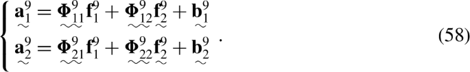
All accelerations are unique because the DCA-based method is applicable for MBSs with ideal constraints. Hence, only the uniqueness of some reactions (that are not underlined) is unknown.
Using Eq. (56), it may be concluded that for bodies \(i\in \{1, 2, 3, 4\}\), the reactions in joints corresponding to the studied sets—namely \(B\), \(D\), \(F\), and \(H\)—are nonunique. The justification is straightforward: if the accelerations are unique, then the reactions \(\mathbf{f}_{i_{2}}\) have to be nonunique since the reactions in the opposite handles \(\mathbf{f}_{i_{1}}\) are nonunique.
A different situation occurs in the cases of bodies 5, 6, and 9. Analyzing Eqs. (57) and (58), it may be concluded that reaction forces \(\mathbf{f}_{i_{2}}\), \(i\in \{5,6\}\), and \(\mathbf{f}_{9_{1}}\) have to be unique since the remaining elements of the mentioned equations of motion are unique or nonsingular. These reactions correspond to spherical joints \(L\), \(N\), and \(Q\). Hence, the reactions in these joints are unique.
The outcomes from this step are shown in Fig. 13.
Fig. 13 
First execution of Step 6.—bodies 1–6 and 9
- Step 7.:
-
Propagate the obtained information inside the binary assembly of the system from the leaves toward the root.
Now, the novel information may be propagated inside the binary assembly. The same reactions act on body 7 (and further subassemblies) that influence bodies 1–6, but they are opposite, while the reaction acting on body 8 is opposite to the reaction that influences body 9 in point \(Q\). This step of the algorithm is illustrated in Fig. 14.
Fig. 14 
Third propagation of the results
- Step 8.:
-
Repeat Step 6. and Step 7. until the uniqueness of all the joint reactions is checked.
-
Step 6. (check the reaction uniqueness of bodies with two nonempty handles, for which the uniqueness of only one joint reaction is unknown).
Now, body 8 may be considered. The situation is analogous to Eq. (58) considered in the first call of Step 6. Hence, the following form of the equation of motion may be obtained:

The results are analogous to the case of body 9—the reaction in spherical joint \(P\) that corresponds to handle \(8_{1}\) is unique. This is presented in Fig. 15.
Fig. 15 
Second execution of Step 6.—body 8
-
Step 7. (propagate the results inside the binary assembly).
The reaction in spherical joint \(P\) is also present at different levels of the assembly, hence, the subsequent propagation of the results should be carried out (in this example, this step is performed for completeness since the uniqueness of all the joint reactions is already known; however, this is not the general case). This step is presented in Fig. 16.
Fig. 16 
Last propagation of the results
-


 , while singular matrices and nonunique vectors are
  ). For the considered MBS, bodies of numbers 1-6 and 9 may be studied in this step.


It may be concluded that the reactions in spherical joints \(A\), \(B\), \(C\), \(D\), \(E\), \(F\), \(G\), and \(H\) are nonunique, while the reactions in spherical joints \(K\), \(L\), \(M\), \(N\), \(P\), \(Q\), and \(R\) are unique. The results are illustrated in Fig. 17, where the joints with unique and nonunique reactions are marked in  and
and  , respectively.

Final results
It may be noted that the obtained results in the parallelogram section of the considered MBS follow the results obtained earlier (see, e.g., [12]), and the reactions in the triple pendulum part are unique, which is in accordance with the intuition (an open kinematic chain has all unique reactions).
When the uniqueness of joint reactions is known, decisions regarding the model need to be made. In our case, some of the reactions are unique, and some are nonunique; hence, the model will be fully flexible or hybrid (partially rigid–partially flexible) to give us realistic reaction forces (see [13] for more details). In the analyzed mechanism, bodies 1, 2, 3, 4, and 7 (with nonunique joint reactions) will be modeled as flexible, while the remaining bodies may be flexible or rigid. After the proper model is built, realistic reaction forces may be calculated in the last stage of the DCA—the back-substitution pass.
5 Conclusions
The problem of the indeterminacy of the reactions, observed when an overconstrained MBS is modeled as a rigid-body system, is considered. In many technical problems, the reaction-uniqueness analysis is crucial for assessing the fidelity of the model and looking for trustworthy solutions.
A novel approach to the reaction-uniqueness analysis is proposed. Unlike the previously available methods, the devised procedure is dedicated to systems described by the relative coordinates. The new approach is based on one of the most effective methods used for dynamic simulations of complex MBSs—the divide-and-conquer algorithm. The proposed approach integrates seamlessly with the DCA framework.
The devised method may be used to assess the joint-reaction uniqueness of holonomic systems with ideal constraints, for which the multijoint connection has to be at most between the complete assembly and the ground. Moreover, matrices \(\mathbf{U}\) must be nonsingular, and the analysis has to be performed in a nonsingular configuration of the MBS.
In the proposed approach, the numerical tools known from the constraint-matrix-based and FBD-based uniqueness tests (namely, the rank-comparison, QR-decomposition, SVD, and nullspace methods) have been applied to one step of the algorithm that was formulated for the DCA-based uniqueness analysis method. In the DCA-based method, not all reactions are tested at the same time. Hence, the discussed method does not destroy the structure of the DCA, and it may be applied to existing codes of this algorithm.
The applicability of the new method was illustrated with the example of a spatial parallelogram mechanism with a triple pendulum. The obtained results corroborate the correctness of the proposed approach. At the present stage of development, the method is quite limited; nevertheless, a broad class of MBSs may be analyzed. Other classes of MBSs constitute potential areas of research.
Data Availability
No datasets were generated or analysed during the current study.
References
Mukherjee, R.M., Crozier, P.S., Plimpton, S.J., Anderson, K.S.: Substructured molecular dynamics using multibody dynamics algorithms. Int. J. Non-Linear Mech. 43(10), 1040–1055 (2008). https://doi.org/10.1016/j.ijnonlinmec.2008.04.003
Malczyk, P., Frączek, J.: Molecular dynamics simulation of simple polymer chain formation using divide and conquer algorithm based on the augmented Lagrangian method. Proc. Inst. Mech. Eng., Proc., Part K, J. Multi-Body Dyn. 229(2), 116–131 (2015). https://doi.org/10.1177/1464419314549875
Curtis, N.: Craniofacial biomechanics: an overview of recent multibody modelling studies. J. Anat. 218(1), 16–25 (2011). https://doi.org/10.1111/j.1469-7580.2010.01317.x
Mazhar, H., Heyn, T., Negrut, D., Tasora, A.: Using Nesterov’s method to accelerate multibody dynamics with friction and contact. ACM Trans. Graph. 34(3), 32–13214 (2015). https://doi.org/10.1145/273562710.1145/2735627
Zierath, J., Woernle, C.: Contact modelling in multibody systems by means of a boundary element co-simulation and a Dirichlet-to-Neumann algorithm. In: Multibody Dynamics. Computational Methods and Applications, pp. 25–52. Springer, Dordrecht (2013). https://doi.org/10.1007/978-94-007-5404-1_2
Pazouki, A., Mazhar, H., Negrut, D.: Parallel collision detection of ellipsoids with applications in large scale multibody dynamics. Math. Comput. Simul. 82(5), 879–894 (2012). https://doi.org/10.1016/j.matcom.2011.11.005
Shao, H., Xu, P., Yao, S., Peng, Y., Li, R., Zhao, S.: Improved multibody dynamics for investigating energy dissipation in train collisions based on scaling laws. Shock Vib. 2016, 3084052 (2016). https://doi.org/10.1155/2016/3084052
Frączek, J., Wojtyra, M.: On the unique solvability of a direct dynamics problem for mechanisms with redundant constraints and Coulomb friction in joints. Mech. Mach. Theory 46(3), 312–334 (2011). https://doi.org/10.1016/j.mechmachtheory.2010.11.003
Ruzzeh, B., Kövecses, J.: A penalty formulation for dynamics analysis of redundant mechanical systems. J. Comput. Nonlinear Dyn. 6(2), 021008 (2011). https://doi.org/10.1115/1.400251010.1115/1.4002510
Pękal, M., Wojtyra, M.: Constraint-matrix-based method for reaction and driving forces uniqueness analysis in overconstrained or overactuated multibody systems. Mech. Mach. Theory 188, 105368 (2023). https://doi.org/10.1016/j.mechmachtheory.2023.105368
Müller, A.: A conservative elimination procedure for permanently redundant closure constraints in MBS-models with relative coordinates. Multibody Syst. Dyn. 16(4), 309–330 (2006). https://doi.org/10.1007/s11044-006-9028-0
Wojtyra, M.: Joint reactions in rigid body mechanisms with dependent constraints. Mech. Mach. Theory 44(12), 2265–2278 (2009). https://doi.org/10.1016/j.mechmachtheory.2009.07.008
Wojtyra, M., Frączek, J.: Joint reactions in rigid or flexible body mechanisms with redundant constraints. Bull. Pol. Acad. Sci., Tech. Sci. 60(3), 617–626 (2012). https://doi.org/10.2478/v10175-012-0073-y
García de Jalón, J., Gutiérrez-López, M.D.: Multibody dynamics with redundant constraints and singular mass matrix: existence, uniqueness, and determination of solutions for accelerations and constraint forces. Multibody Syst. Dyn. 30(3), 311–341 (2013). https://doi.org/10.1007/s11044-013-9358-7
González, F., Kövecses, J.: Use of penalty formulations in dynamic simulation and analysis of redundantly constrained multibody systems. Multibody Syst. Dyn. 29(1), 57–76 (2013). https://doi.org/10.1007/s11044-012-9322-y
Shang, H., Wei, D., Kang, R., Chen, Y.: A deployable robot based on the Bricard linkage. In: Zhang, X., Wang, N., Huang, Y. (eds.) Mechanism and Machine Science. Proceedings of Asian MMS 2016 & CCMMS 2016. Lecture Notes in Electrical Engineering, vol. 408, pp. 737–747. Springer, Singapore (2017). https://doi.org/10.1007/978-981-10-2875-5_61
Müller, A.: Elimination of redundant cut joint constraints for multibody system models. J. Mech. Des. 126(3), 488–494 (2004). https://doi.org/10.1115/1.173737710.1115/1.1737377
Chen, Y.: Design of Structural Mechanisms. PhD Thesis, University of Oxford, Oxford (2003)
Uicker, J.J. Jr., Pennock, G.R., Shigley, J.E.: Theory of Machines and Mechanisms, 3rd edn. Oxford University Press, New York (2003)
Mariti, L., Belfiore, N.P., Pennestrì, E., Valentini, P.P.: Comparison of solution strategies for multibody dynamics equations. Int. J. Numer. Methods Eng. 88(7), 637–656 (2011). https://doi.org/10.1002/nme.319010.1002/nme.3190
Pękal, M., Frączek, J.: Comparison of selected formulations for multibody system dynamics with redundant constraints. Arch. Mech. Eng. 63(1), 93–112 (2016). https://doi.org/10.1515/meceng-2016-0005
Pękal, M., Frączek, J.: Comparison of natural complement formulations for multibody dynamics. J. Theor. Appl. Mech. 54(4), 1391–1404 (2016). https://doi.org/10.15632/jtam-pl.54.4.1391
Wojtyra, M.: Joint reaction forces in multibody systems with redundant constraints. Multibody Syst. Dyn. 14(1), 23–46 (2005). https://doi.org/10.1007/s11044-005-5967-0
Featherstone, R.: Rigid Body Dynamics Algorithms. Springer, New York (2008). https://doi.org/10.1007/978-1-4899-7560-7
Featherstone, R., Orin, D.E.: Dynamics. In: Siciliano, B., Khatib, O. (eds.) Springer Handbook of Robotics, pp. 35–65. Springer, Berlin (2008). https://doi.org/10.1007/978-3-540-30301-5_3
Pękal, M., Wojtyra, M., Frączek, J.: Free-body-diagram method for the uniqueness analysis of reactions and driving forces in redundantly constrained multibody systems with nonholonomic constraints. Mech. Mach. Theory 133, 329–346 (2019). https://doi.org/10.1016/j.mechmachtheory.2018.11.021
Wojtyra, M., Frączek, J.: Solvability of reactions in rigid multibody systems with redundant nonholonomic constraints. Multibody Syst. Dyn. 30(2), 153–171 (2013). https://doi.org/10.1007/s11044-013-9352-0
Wojtyra, M., Frączek, J.: Comparison of selected methods of handling redundant constraints in multibody systems simulations. J. Comput. Nonlinear Dyn. 8(2), 021007 (2013). https://doi.org/10.1115/1.400695810.1115/1.4006958
Callejo, A., Gholami, F., Enzenhöfer, A., Kövecses, J.: Unique minimum norm solution to redundant reaction forces in multibody systems. Mech. Mach. Theory 116, 310–325 (2017). https://doi.org/10.1016/j.mechmachtheory.2017.06.001
Šalinić, S.: Determination of joint reaction forces in a symbolic form in rigid multibody systems. Mech. Mach. Theory 46(11), 1796–1810 (2011). https://doi.org/10.1016/j.mechmachtheory.2011.06.006
Khalil, H.K.: Nonlinear Systems, 3rd edn. Pearson Education Limited, Harlow (2014)
Song, S.-M., Gao, X.: The mobility equation and the solvability of joint forces/torques in dynamic analysis. J. Mech. Des. 114(2), 257–262 (1992). https://doi.org/10.1115/1.291694010.1115/1.2916940
Pękal, M., Frączek, J., Tomulik, P.: Solvability of reactions and inverse dynamics problem for complex kinematic chains. In: The 21st International Conference on Methods and Models in Automation and Robotics, Międzyzdroje, Poland (2016). https://doi.org/10.1109/MMAR.2016.7575078
Pękal, M., Frączek, J.: A kinetostatics-based study of uniqueness of reactions and drives in robotics. J. Autom. Mob. Robot. Intell. Syst. 11(2), 21–30 (2017). https://doi.org/10.14313/JAMRIS_2-2017/13
Featherstone, R.: A divide-and-conquer articulated-body algorithm for parallel O(log(n)) calculation of rigid-body dynamics. Part 1: basic algorithm. Int. J. Robot. Res. 18(9), 867–875 (1999). https://doi.org/10.1177/02783649922066619
Featherstone, R.: A divide-and-conquer articulated-body algorithm for parallel O(log(n)) calculation of rigid-body dynamics. Part 2: trees, loops, and accuracy. Int. J. Robot. Res. 18(9), 876–892 (1999). https://doi.org/10.1177/02783649922066628
Malczyk, P., Frączek, J.: A divide and conquer algorithm for constrained multibody system dynamics based on augmented Lagrangian method with projections-based error correction. Nonlinear Dyn. 70(1), 871–889 (2012). https://doi.org/10.1007/s11071-012-0503-2
Laflin, J.J., Anderson, K.S., Khan, I.M., Poursina, M.: Advances in the application of the divide-and-conquer algorithm to multibody system dynamics. J. Comput. Nonlinear Dyn. 9(4), 041003 (2014). https://doi.org/10.1115/1.402607210.1115/1.4026072
Laflin, J.J., Anderson, K.S., Khan, I.M., Poursina, M.: New and extended applications of the divide-and-conquer algorithm for multibody dynamics. J. Comput. Nonlinear Dyn. 9(4), 041004 (2014). https://doi.org/10.1115/1.402786910.1115/1.4027869
Laflin, J.J., Anderson, K.S.: Geometrically exact beam equations in the adaptive DCA framework. Part 1: static example. Multibody Syst. Dyn. 47, 1–19 (2019). https://doi.org/10.1007/s11044-019-09669-1
Kingsley, C., Poursina, M.: Extension of the divide-and-conquer algorithm for the efficient inverse dynamics analysis of multibody systems. Multibody Syst. Dyn. 42(2), 145–167 (2018). https://doi.org/10.1007/s11044-017-9591-6
Malczyk, P., Frączek, J., González, F., Cuadrado, J.: Index-3 divide-and-conquer algorithm for efficient multibody system dynamics simulations: theory and parallel implementation. Nonlinear Dyn. 95(1), 727–747 (2019). https://doi.org/10.1007/s11071-018-4593-3
Turno, S., Malczyk, P.: FPGA acceleration of planar multibody dynamics simulations in the Hamiltonian–based divide–and–conquer framework. Multibody Syst. Dyn. 57, 25–53 (2022). https://doi.org/10.1007/s11044-022-09860-x
Pękal, M.: Uniqueness analysis of constraint and driving forces in multibody models of mechanical and robotic systems (in Polish). PhD Thesis, Warsaw University of Technology, Warsaw (2019)
Golub, G.H., Van Loan, C.F.: Matrix Computations, 3rd edn. The Johns Hopkins University Press, Baltimore, London (1996)
Strang, G., Borre, K.: Linear Algebra, Geodesy, and GPS. Wellesley-Cambridge Press, Wellesley (1997)
Acknowledgements
For the purpose of Open Access, the authors have applied a CC-BY public copyright license to any Author Accepted Manuscript (AAM) version arising from this submission.
Funding
This work has been supported by the National Science Centre, Poland under grant no. 2022/45/B/ST8/00661.
Author information
Authors and Affiliations
Contributions
All authors worked on the concept. M.P., P.M., and M.W. prepared the state-of-the-art analysis and developed the method. M.P. wrote the manuscript draft and prepared figures. P.M. and M.W. checked the algorithm and edited the manuscript. All authors reviewed the manuscript.
Corresponding author
Ethics declarations
Competing interests
J.F. is a member of the Advisory Board of the journal Multibody System Dynamics.
Additional information
Publisher’s Note
Springer Nature remains neutral with regard to jurisdictional claims in published maps and institutional affiliations.
Rights and permissions
Open Access This article is licensed under a Creative Commons Attribution 4.0 International License, which permits use, sharing, adaptation, distribution and reproduction in any medium or format, as long as you give appropriate credit to the original author(s) and the source, provide a link to the Creative Commons licence, and indicate if changes were made. The images or other third party material in this article are included in the article’s Creative Commons licence, unless indicated otherwise in a credit line to the material. If material is not included in the article’s Creative Commons licence and your intended use is not permitted by statutory regulation or exceeds the permitted use, you will need to obtain permission directly from the copyright holder. To view a copy of this licence, visit http://creativecommons.org/licenses/by/4.0/.
About this article

Cite this article
Pękal, M., Malczyk, P., Wojtyra, M. et al. Divide-and-conquer-based approach for the reaction uniqueness analysis in overconstrained multibody systems. Multibody Syst Dyn (2024). https://doi.org/10.1007/s11044-024-10013-5
Received:
Accepted:
Published:
DOI: https://doi.org/10.1007/s11044-024-10013-5