
Abstract
A nonlinear amensalism model of the form
where \(r_{i}, P_{i}, u, i=1, 2, \alpha_{1}, \alpha_{2}, \alpha_{3}\) are all positive constants, is proposed and studied in this paper. The dynamic behaviors of the system are determined by the sign of the term \(1-u (\frac{P_{2}}{P_{1}} )^{\alpha_{2}} \). If \(1-u (\frac {P_{2}}{P_{1}} )^{\alpha_{2}}>0\), then the unique positive equilibrium \(D(N_{1}^{*},N_{2}^{*})\) is globally attractive, if \(1-u (\frac{P_{2}}{P_{1}} )^{\alpha_{2}}<0\), then the boundary equilibrium \(C(0, P_{2})\) is globally attractive. Our results supplement and complement the main results of Xiong, Wang, and Zhang (Advances in Applied Mathematics 5(2):255–261, 2016).
1 Introduction
During the last decade, many scholars [1–12] investigated the dynamic behaviors of the amensalism model; here, amensalism means that a species inflicts harm to other species without any costs or benefits received by the other. Such topics as the stability of the equilibrium [1, 3–8], the existence of the positive periodic solution [2, 9, 11], the extinction of the species [8, 10], the influence of the cover [8, 12], the influence of the functional response [10], etc. have been extensively studied. Recently, Xiong et al. [1] proposed the following amensalism model:
where \(r_{i}, P_{i}, u, i=1, 2\), are all positive constants. They investigated the local stability property of the equilibria of system (1.1).
On the other hand, in 1973, in their study on the validity of the competition modeling, Ayala et al. [13] found that the following nonlinear competition model accounts best for the experimental results:
Since then, the dynamic behaviors of the nonlinear competition system and nonlinear competition-predator-prey system have been extensively studied by many scholars [13–30]. Such topics as the persistence [14, 17, 20, 23], extinction [15, 17–19, 26, 28, 30], the stability of the equilibrium [19–22], the existence and stability of the periodic solution [18, 22, 24, 25, 29], etc. have been extensively investigated, and many excellent results have been obtained.
It brings to our attention that to this day, there is still no scholar to propose and investigate the nonlinear amensalism model. Stimulated by the works of Xiong et al. [1], Chen et al. [14, 15], Lu et al. [23], Lu [24], and Wang [26], in this paper, we propose the following nonlinear amensalism model:
where \(r_{i}, P_{i}, u, i=1, 2, \alpha_{j}, j=1, 2, 3\), are all positive constants.
As far as system (1.3) is concerned, one interesting issue is:
Find out the influence of the parameter \(\alpha_{i}\), \(i=1, 2, 3\), which reflects the influence of the nonlinearity.
The paper is arranged as follows. We investigate the existence and local stability property of the equilibrium solutions of system (1.3) in the next section. In Sect. 3, by applying the differential inequality theory, we investigate the global stability property of the equilibria. The influence of the parameter \(\alpha_{i}, i=1, 2, 3\), is then discussed in Sect. 4. Some examples together with their numeric simulations are presented in Sect. 5 to show the feasibility of the main results. We end this paper with a brief discussion.
2 Local stability
The system always admits three boundary equilibria \(A(0,0)\), \(B(P_{1}, 0)\), \(C(0, P_{2})\). Also, if \(1> u (\frac{P_{2}}{P_{1}} )^{\alpha_{2}}\), the system admits a unique positive equilibrium
We shall now investigate the local stability property of the above equilibria.
The variational matrix of the system of Eq. (1.3) is
where
Theorem 2.1
Assume that \(\alpha_{2}\geq1\), then
-
(1)
\(A(0,0)\) is unstable;
-
(2)
\(B(P_{1}, 0) \) is a saddle point, thus, is unstable;
-
(3)
if \(1-u (\frac{P_{2}}{P_{1}} )^{\alpha_{2}}>0\), \(C(0, P_{2})\) is a saddle point and consequently unstable; if \(1-u (\frac{P_{2}}{P_{1}} )^{\alpha_{2}}<0\), \(C(0, P_{2})\) is a stable node;
-
(4)
if \(1-u (\frac{P_{2}}{P_{1}} )^{\alpha_{2}}>0\), \(D(N_{1}^{*},N_{2}^{*})\) is a stable node.
Remark 2.1
If \(\alpha_{i}=1\), \(i=1, 2, 3\), then Theorem 2.1 degenerates to the main result of Xiong et al. [1], hence, we generalize the main result of [1]. Note that the boundary equilibria are independent of \(\alpha_{i}, i=1, 2, 3\), hence, \(\alpha_{i}\), \(i=1, 3\), has no influence on the existence and stability of the boundary equilibria.
Remark 2.2
From (2.1), the second term in \(J(N_{1}, N_{2})\) is \(-\frac{r_{1}uN_{1}\alpha_{2}N_{2}^{\alpha_{2}-1}}{P_{1}^{\alpha _{2}}}\), which means that if \(\alpha_{2}<1\), then at \(N_{2}=0\), the value of this term could not be computed. Hence, for \(0<\alpha_{2}<1\) case, the local stability of the equilibrium \(A(0,0)\) and \(B(P_{1}, 0)\) could not be determined by analyzing the Jacobian matrix.
Proof of Theorem 2.1
(1) From (2.1) we could see that the Jacobian of the system about the equilibrium point \(A(0,0)\) is given by
The eigenvalues of the matrix are \(\lambda_{1}=r_{1}>0, \lambda_{2}=r_{2}>0\). Hence, \(A(0,0)\) is unstable;
(2) The Jacobian of the system about the equilibrium point \(B(P_{1},0)\) is given by
The eigenvalues of the matrix are \(\lambda_{1}=-r_{1}\alpha_{1}<0, \lambda_{2}= r_{2}>0\). So \(B(P_{1}, 0)\) is a saddle point, it is unstable;
(3) The Jacobian of the system about the equilibrium point \(C(0,P_{2})\) is given by
The two eigenvalues of the matrix satisfy \(\lambda_{1}=r_{1} (1-u (\frac{P_{2}}{P_{1}} )^{\alpha_{2}} ), \lambda_{2}=-r_{2}\alpha_{3}<0\). Obviously, if \(1-u (\frac{P_{2}}{P_{1}} )^{\alpha_{2}}>0\), then \(\lambda _{1}>0\); and consequently, \(C(0, P_{2})\) is a saddle point, it is unstable; if \(1-u (\frac {P_{2}}{P_{1}} )^{\alpha_{2}}<0\), then \(\lambda_{1}<0\), \(C(0, P_{2})\) is locally stable, it is a stable node.
(4) Note that the positive equilibrium \(D(N_{1}^{*}, N_{2}^{*})\) satisfies
Combining with (2.1) and (2.5), we could see that the Jacobian of the system about the equilibrium point \(D(N_{1}^{*},N_{2}^{*})\) is given by
The eigenvalues of the variational matrix (2.6) is the roots \(\lambda_{1}=-r_{1} (\frac{N_{1}^{*}}{P_{1}} )^{\alpha_{1}}\alpha_{1}<0\), \(\lambda_{2}=- r_{2} (\frac{N_{2}^{*}}{P_{2}} )^{\alpha_{3}}\alpha_{3}<0\). Thus, \(D(N_{1}^{*}, N_{2}^{*})\) is locally stable.
The proof of Theorem 2.1 is finished. □
3 Global stability
As was pointed out in the previous section, for the case \(\alpha_{2}<1\), the local stability property of the boundary equilibrium \(A(0,0)\) and \(B(P_{1},0)\) could not be determined by using the Jacobian matrix (2.1). The aim of this section is to try to solve this problem and to further investigate the global stability property of the equilibria of system (1.3).
Lemma 3.1
Consider the system
where \(r_{2}, P_{2}, \alpha_{3}\) are all positive constants. The unique positive equilibrium \(N_{2}^{*}=P_{2}\) of system (3.1) is globally stable.
Proof
Set
then
hence \(F(N_{2})=0\) has at least one positive solution on the interval \((0,+\infty)\). Also, for \(N_{2}\geq0\), from (3.2)
Hence, \(F(N_{2})\) is strictly decreasing on the interval \((0,+\infty)\), therefore, \(F(N_{2})=0\) has at most one positive solution on the interval \((0,+\infty)\). One could easily see that \(N_{2}=P_{2}\) is the solution of (3.2). The above analysis shows that \(N_{2}^{*}=P_{2}\) is the unique positive equilibrium of system (3.1).
On the other hand, from the above analysis, we also have
-
(i)
For all \(N_{2}^{*} > N_{2} > 0, F(N_{2}) > 0\).
-
(ii)
For all \(N_{2} > N_{2}^{*} > 0, F(N_{2}) < 0\).
Hence, it immediately follows from Theorem 2.1 of [27] that the unique positive equilibrium \(N_{2}^{*}\) of system (3.1) is globally stable. □
The next lemma is a direct corollary of Lemma 2.2 of Chen [16].
Lemma 3.2
If \(a>0, b>0\), and \(\dot{x}\geq x(b-ax^{\alpha})\), where α is some positive constant, when \(t\geq{0}\) and \(x(0)>0\), we have
If \(a>0\), \(b>0\), and \(\dot{x}\leq x(b-ax^{\alpha})\), where α is some positive constant, when \(t\geq{0}\) and \(x(0)>0\), we have
Theorem 3.1
-
(a)
Assume that \(1-u (\frac{P_{2}}{P_{1}} )^{\alpha_{2}}<0\), then \(C(0, P_{2})\) is globally attractive;
-
(b)
Assume that \(1-u (\frac{P_{2}}{P_{1}} )^{\alpha_{2}}>0\), then \(D(N_{1}^{*},N_{2}^{*})\) is globally attractive.
Proof
(a) Condition \(1-u (\frac{P_{2}}{P_{1}} )^{\alpha_{2}}<0\) implies that for enough small positive constant \(\varepsilon>0\) (\(\varepsilon<\frac {1}{2}P_{2}\)), the following inequality holds:
Let \((N_{1}(t), N_{2}(t))\) be any positive solution of system (1.3). It follows from Lemma 3.1 that
For \(\varepsilon>0\) which satisfies (3.3), from (3.4) there exists an enough large \(T_{1}\) such that
Since function \(y=x^{\alpha_{2}}\) is strictly increasing for all \(x>0\), it follows from (3.5) that
For \(t\geq T_{1}\), from the right-hand side of (3.5) and the first equation of system (1.3), one has
Equation (3.7) together with (3.1) leads to
(b) Condition \(1-u (\frac{P_{2}}{P_{1}} )^{\alpha_{2}}>0\) implies that for enough small positive constant \(\varepsilon>0\) (\(\varepsilon<\frac {1}{2}P_{2}\)), the following inequality holds:
Let \((N_{1}(t), N_{2}(t))\) be any positive solution of system (1.3), it follows from Lemma 3.1 that
For \(\varepsilon>0\) which satisfies (3.8), from (3.9) there exists an enough large \(T_{2}\) such that
For \(t\geq T_{2}\), from the left-hand side of (3.10) and the first equation of system (1.3), one has
Applying Lemma 3.2 to (3.11), we could obtain
Since ε is an arbitrary small positive constant, setting \(\varepsilon\rightarrow0\) leads to
For \(t\geq T_{2}\), from the right-hand side of (3.10) and the first equation of system (1.3), one has
Applying Lemma 3.2 to (3.14), we could obtain
Since ε is an arbitrary small positive constant, setting \(\varepsilon\rightarrow0\) leads to
Equation (3.13) together with (3.16) leads to
This ends the proof of Theorem 3.1. □
Remark 3.1
Theorems 2.1 and 3.1 show that if system (1.3) admits the unique positive equilibrium, then the positive equilibrium is globally attractive.
Remark 3.2
Noting that if \(C(0,P_{2})\) or \(D(N_{1}^{*}, N_{2}^{*})\) is globally attractive, then all the solutions with positive initial conditions will finally asymptotically to the equilibrium, which means that the solutions with positive solution could not be asymptotically to \(A(0,0)\) and \(B(P_{1},0)\), thus, \(A(0,0)\) and \(B(P_{1},0)\) is unstable. Theorem 3.1 shows that for almost all the cases (only \(1-u (\frac{P_{2}}{P_{1}} )^{\alpha_{2}}=0\) could not be determined), \(A(0,0)\) and \(B(P_{1},0)\) are unstable.
Remark 3.3
Xiong et al. [1] proposed system (1.1) and investigated the local stability property of the equilibria. However, they did not give any information about the global stability property of the equilibrium. Thus, Theorem 3.1 can be seen as the supplement of the main result of [1].
4 The influence of the parameter \(\alpha_{i}\)
Now let us consider the influence of the parameter \(\alpha _{i}, i=1, 2, 3\), on the finial density of the two species. We will focus our attention on the positive equilibrium. Noting that
\(N_{2}^{*}=P_{2}\) is independent of the parameter \(\alpha_{i}\), hence, \(\alpha _{i}\) has no influence on the final density of the second species. However, \(N_{1}^{*}\) is the function of the parameters \(\alpha_{1} \) and \(\alpha_{2}\), hence, it is necessary to investigate the relationship of \(N_{1}^{*}\) and \(\alpha_{i}\), \(i= 1, 2\). Noting that
hence, \(N_{1}^{*}\) is the increasing function of \(\alpha_{1}\).
thus
-
(1)
If \(P_{2} >P_{1} \), then \(\frac{\partial N_{1}^{*}}{\partial\alpha_{2}}<0\), and \(N_{1}^{*}\) is the strictly decreasing function of \(\alpha_{2}\);
-
(2)
If \(P_{2} < P_{1}\), then \(\frac{\partial N_{1}^{*}}{\partial\alpha_{2}}>0\), and \(N_{1}^{*}\) is the strictly increasing function of \(\alpha_{2}\).
-
(3)
If \(P_{2}=P_{1}\), then \(\frac{\partial N_{1}^{*}}{\partial\alpha_{2}}=0\), and \(N_{1}^{*}\) is independent of \(\alpha_{2}\).
5 Numeric simulations
Example 5.1
Consider the following amensalism system:
Here, corresponding to system (1.3), we take \(r_{1}=r_{2}=P_{2}=1\), \(\alpha_{2}=2\), \(P_{1}=2\), \(\alpha_{3}=\alpha_{1}=1\), \(u=1\). One could easily check that
So, from Theorem 3.1, the unique positive equilibrium \(D(1.5,1)\) is globally attractive. Figure 1 also supports this assertion.

Numeric simulations of system (5.1), the initial conditions \((x(0), y(0))=(0.4,5), (1,5), (1, 0.02), (1.5,5), (5,5), (5,0.2)\), and \((5,3)\), respectively
Example 5.2
Consider the following amensalism system:
Here, corresponding to system (1.3), we take \(r_{1}=r_{2}=P_{1}=1\), \(\alpha_{2}=2\), \(P_{2}=2\), \(\alpha_{3}=\alpha_{1}=1\), \(u=1\). One could easily check that
So, from Theorem 3.1, the boundary equilibrium \(C(0,2)\) is globally attractive. Figure 2 also supports this assertion.

Numeric simulations of system (5.2), the initial conditions \((x(0), y(0))=(0.4,5), (5,1), (5, 3), (5,5)\), and \((5,0.2)\), respectively
Example 5.3
Consider the following amensalism system:
Here, corresponding to system (1.3), we take \(r_{1}=r_{2}=P_{1}=1\), \(\alpha_{2}=2\), \(P_{2}=1\), \(\alpha_{3}=\alpha_{1}=1\), \(u=1\). One could easily check that
Numeric simulation (Fig. 3) shows that in this case the boundary equilibrium \(C(0,1)\) is globally asymptotically stable.

Numeric simulations of system (5.3), the initial conditions \((x(0), y(0))=(1,5), (0.1,0.002), (1.5, 5), (5,5), (5,3)\), and \((5,0.2)\), respectively
Example 5.4
Consider the function
-
(1)
Let us take \(P_{1}=1, P_{2}=2, \alpha_{2}=1, u=\frac{1}{4}\). From Sect. 4 we know that \(N_{1}^{*}\) is the strictly increasing function of \(\alpha_{1}\). Figure 4 also supports this assertion;
Figure 4 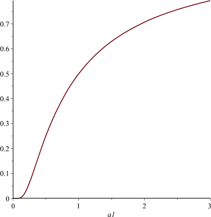
The relationship of \(N_{1}^{*}\) and \(\alpha_{1}\), here we choose \(P_{1}=1\), \(P2=2\), \(\alpha_{2}=1\)
-
(2)
Let us take \(P_{1}=1, P_{2}=2, \alpha_{1}=1, u=\frac{1}{4}\). From Sect. 4 we know that \(N_{1}^{*}\) is the strictly decreasing function of \(\alpha_{2}\). Figure 5 also supports this assertion;
Figure 5 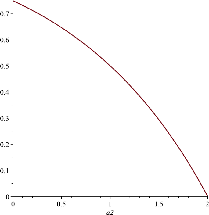
The relationship of \(N_{1}^{*}\) and \(\alpha_{2}\), here we choose \(P_{1}=1\), \(P_{2}=2\), \(\alpha_{1}=1\)
-
(3)
Let us take \(P_{1}=1, P_{2}=\frac{1}{2}, \alpha_{1}=1, u=\frac{1}{4}\). From Sect. 4 we know that \(N_{1}^{*}\) is the strictly increasing function of \(\alpha_{2}\). Figure 6 also supports this assertion;
Figure 6 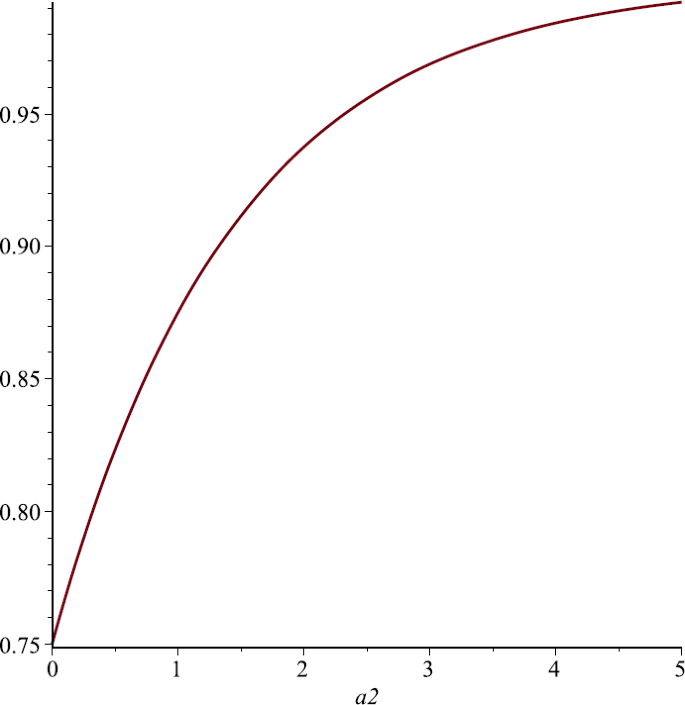
The relationship of \(N_{1}^{*}\) and \(\alpha_{2}\), here we choose \(P_{1}=1\), \(P_{2}=\frac{1}{2}\)
-
(4)
Let us take \(P_{1}=1, P_{2}=1, \alpha_{1}=1, u=\frac{1}{4}\). From Sect. 4 we know that \(N_{1}^{*}\) is independent of \(\alpha_{2}\). Figure 7 also supports this assertion.
Figure 7 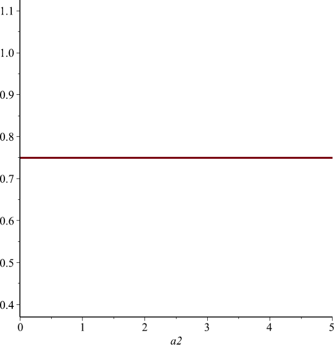
The relationship of \(N_{1}^{*}\) and \(\alpha_{2}\), here we choose \(P_{1}=P_{2}=1\)


6 Discussion
Stimulated by the works of Xiong et al. [1] and Chen et al. [14–19], in this paper, we propose the nonlinear amensalism model (1.3).
We first investigated the local stability property of the equilibria, and we found that, by introducing the nonlinear term, the situation became complicated, and only under the assumption \(\alpha _{2}\geq1\) could we give the local stability result of \(A(0,0)\) and \(B(P_{1},0)\). To overcome this difficulty, we used the differential inequality theory, and finally proved the following results: if the positive equilibrium exists, then it is globally attractive.
We also investigated the relationship among \(N_{1}^{*}\) and \(\alpha _{i}\), and found that \(\alpha_{2}\) and the ratio of \(\frac{P_{2}}{P_{1}}\) play most important roles on the final density of the first species.
We mention here that we did not discuss the degenerate case
However, numeric simulation (Fig. 3) shows that in this case, the boundary equilibrium \(C(0, P2)\) is globally asymptotically stable. For fixed \(\alpha_{i}, i=1, 2, 3\), we could put forward some progress, such as numeric simulation, on this direction. However, we still have difficulty obtaining the analysis result, we leave this for the future investigation.
References
Xiong, H.H., Wang, B.B., Zhang, H.L.: Stability analysis on the dynamic model of fish swarm amensalism. Adv. Appl. Math. 5(2), 255–261 (2016)
Han, R.Y., Xue, Y.L., Yang, L.Y., et al.: On the existence of positive periodic solution of a Lotka–Volterra amensalism model. J. Rongyang Univ. 33(2), 22–26 (2015)
Chen, B.G.: Dynamic behaviors of a non-selective harvesting Lotka–Volterra amensalism model incorporating partial closure for the populations. Adv. Differ. Equ. 2018, 111 (2018)
Zhu, Z.F., Chen, Q.L.: Mathematic analysis on commensalism Lotka–Volterra model of populations. J. Jixi Univ. 8(5), 100–101 (2008)
Zhang, Z.: Stability and bifurcation analysis for a amensalism system with delays. Math. Numer. Sin. 30, 213–224 (2008)
Sita Rambabu, B., Narayan, K.L., Bathul, S.: A mathematical study of two species amensalism model with a cover for the first species by homotopy analysis method. Adv. Appl. Sci. Res. 3(3), 1821–1826 (2012)
Acharyulu, K.V.L.N., Pattabhi Ramacharyulu, N.Ch.: On the carrying capacity of enemy species, inhibition coefficient of amensal species and dominance reversal time in an ecological amensalism -a special case study with numerical approach. Int. J. Adv. Sci. Technol. 43, 49–57 (2012)
Xie, X.D., Chen, F.D., He, M.X.: Dynamic behaviors of two species amensalism model with a cover for the first species. J. Math. Computer Sci. 16, 395–401 (2016)
Lin, Q.X., Zhou, X.Y.: On the existence of positive periodic solution of a amensalism model with Holling II functional response. Commun. Math. Biol. Neurosci. 2017, Article ID 3 (2017)
Chen, J.H., Wu, R.X.: A two species amensalism model with non-monotonic functional response. Commun. Math. Biol. Neurosci. 2016, Article ID 19 (2016)
Chen, F.D., Pu, L.Q., Yang, L.Y.: Positive periodic solution of a discrete obligate Lotka–Volterra model. Commun. Math. Biol. Neurosci. 2015, Article ID 14 (2015)
Wu, R.X., Zhao, L., Lin, Q.X.: Stability analysis of a two species amensalism model with Holling II functional response and a cover for the first species. J. Nonlinear Funct. Anal. 2016, Article ID 46 (2016)
Ayala, F.J., Gilpin, M.E., Eherenfeld, J.G.: Competition between species: theoretical models and experimental tests. Theor. Popul. Biol. 4, 331–356 (1973)
Chen, F., Chen, X., Huang, S.: Extinction of a two species non-autonomous competitive system with Beddington–DeAngelis functional response and the effect of toxic substances. Open Math. 14(1), 1157–1173 (2016)
Chen, F.D., Xie, X.D., Miao, Z.S., Pu, L.Q.: Extinction in two species nonautonomous nonlinear competitive system. Appl. Math. Comput. 274, 119–124 (2016)
Chen, F.D., Xie, X.D.: Study on the Dynamic Behaviors of Cooperation Population Modeling. Science Press, Beijing (2014)
Pu, L., Xie, X., Chen, F., et al.: Extinction in two-species nonlinear discrete competitive system. Discrete Dyn. Nat. Soc. 2016, Article ID 2806405 (2016)
Li, Z., Chen, F.: Extinction and almost periodic solutions of a discrete Gilpin–Ayala type population model. J. Differ. Equ. Appl. 19(5), 719–737 (2013)
Ma, Z.Z., Chen, F., Wu, C., Chen, W.: Dynamic behaviors of a Lotka–Volterra predator-prey model incorporating a prey refuge and predator mutual interference. Appl. Math. Comput. 219(15), 7945–7953 (2013)
Li, Z., Chen, F.D., He, M.X.: Asymptotic behavior of the reaction-diffusion model of plankton allelopathy with nonlocal delays. Nonlinear Anal., Real World Appl. 12(3), 1748–1758 (2011)
Chen, L.J., Chen, F.D., Wang, Y.Q.: Influence of predator mutual interference and prey refuge on Lotka–Volterra predator–prey dynamics. Commun. Nonlinear Sci. Numer. Simul. 18(11), 3174–3180 (2013)
Yang, K., Miao, Z., Chen, F., et al.: Influence of single feedback control variable on an autonomous Holling-II type cooperative system. J. Math. Anal. Appl. 435(1), 874–888 (2016)
Lu, H.Y., Yu, G.: Permanence of a Gilpin–Ayala predator-prey system with time-dependent delay. Adv. Differ. Equ. 2015, 109 (2015)
Lu, H.Y.: Periodicity and stability of an impulsive nonlinear competition model with infinitely distributed delays and feedback controls. Adv. Differ. Equ. 2016, 282 (2016)
Zhao, K.H., Ren, Y.P.: Existence of positive periodic solutions for a class of Gilpin–Ayala ecological models with discrete and distributed time delays. Adv. Differ. Equ. 2017, 331 (2017)
Wang, D.H.: Dynamic behaviors of an obligate Gilpin–Ayala system. Adv. Differ. Equ. 2016, 270 (2016)
Chen, L.S.: Mathematical Models and Methods in Ecology. Science Press, Beijing (1988) (in Chinese)
He, M.X., Li, Z., Chen, F.D.: Permanence, extinction and global attractivity of the periodic Gilpin–Ayala competition system with impulses. Nonlinear Anal., Real World Appl. 11(3), 1537–1551 (2010)
Li, Z., Chen, F., He, M.X.: Permanence and global attractivity of a periodic predator-prey system with mutual interference and impulses. Commun. Nonlinear Sci. Numer. Simul. 17(1), 444–453 (2012)
Shi, C.L., Li, Z., Chen, F.D.: Extinction in a nonautonomous Lotka–Volterra competitive system with infinite delay and feedback controls. Nonlinear Anal., Real World Appl. 13(5), 2214–2226 (2012)
Acknowledgements
The author is grateful to the anonymous referees for their excellent suggestions, which greatly improved the presentation of the paper. The research was supported by the National Natural Science Foundation of China under Grant (11601085) and the Natural Science Foundation of Fujian Province (2017J01400).
Author information
Authors and Affiliations
Contributions
All authors contributed equally to the writing of this paper. All authors read and approved the final manuscript.
Corresponding author
Ethics declarations
Competing interests
The author declares that there is no conflict of interests.
Additional information
Publisher’s Note
Springer Nature remains neutral with regard to jurisdictional claims in published maps and institutional affiliations.
Rights and permissions
Open Access This article is distributed under the terms of the Creative Commons Attribution 4.0 International License (http://creativecommons.org/licenses/by/4.0/), which permits unrestricted use, distribution, and reproduction in any medium, provided you give appropriate credit to the original author(s) and the source, provide a link to the Creative Commons license, and indicate if changes were made.
About this article

Cite this article
Wu, R. Dynamic behaviors of a nonlinear amensalism model. Adv Differ Equ 2018, 187 (2018). https://doi.org/10.1186/s13662-018-1624-9
Received:
Accepted:
Published:
DOI: https://doi.org/10.1186/s13662-018-1624-9